Since our last update, the US Federal Reserve, European Central Bank, the People’s Bank of China and other central banks have reduced key policy rates with markets pricing further easing to come. With a coordinated easing cycle now underway, the risk of slowing growth tipping over into recession appears to have diminished.

This has set the scene for strong returns across most equity and fixed income markets, especially in areas where risk premia were previously elevated.

As a result, our current Capital Market Assumptions (30 September 2024) indicate low expected returns overall. We anticipate that a traditional 60% global equity, 40% global government bond portfolio, hedged into US dollars, will deliver a nominal annualised return of 3.8% over the next decade. While opportunities to achieve higher returns exist by reallocating within and across equity and fixed income sectors, the potential return uplift appears to have diminished.

We continue to see a strong need for value-add from asset allocation and security selection decisions as well as from identifying investments that will benefit from structural growth tailwinds to achieve investment objectives.

Forecasts are inherently limited and modelling involves risks, assumptions and uncertainties, they are forward looking and are not guarantees nor a reliable indicator of future results. Actual returns could be materially higher or lower than projected. This information is not intended as a recommendation to invest in any particular asset class or strategy or as a promise of future performance.

Source: Ninety One proprietary Capital Market Assumptions as at 30 September 2024.
These estimates are gross of fees (returns can be reduced by management fees and other expenses incurred) and reflect the view of Ninety One’s multi-asset team, whilst the views of other teams across Ninety One may differ. Details on our Capital Market Assumptions methodology available upon request.

Long-term predictions are fraught with uncertainty and open to error. However, we can retrospectively apply our framework to assess its historical effectiveness. Because we focus on contextual information, we tend to evaluate effectiveness in terms of the reliability of the direction of the signal at market peaks or troughs. Accurately predicting the broad direction over a decade is crucial to achieving favourable investment outcomes.

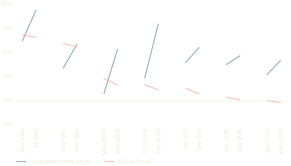
The figure below highlights various market peaks and subsequent troughs, dating back to 1980, for developed market equities and global bonds¹. It also shows the predicted 10-year returns at each of these points.

Figure 1: Expected returns can vary significantly depending on the point of the cycle

Source: Ninety One. Data is global since 2000; prior dates based on US outcomes. Bonds based on 10-year tenor.

For example, the first point on the previous chart corresponds to November 1980 (roughly a market peak) followed by a trough in July of 1982. The relevant 10-year forecasts in each instance were:

Indeed, global equities tripled in the decade from November 1980, and rose fourfold from July 1982. The chart illustrates the desired pattern – riskier assets generally have lower anticipated 10-year returns at market peaks than at subsequent troughs, while the more defensive bond asset tends to perform better at peaks than troughs. Interestingly, although this pattern is repeated over time, it appears to be becoming more compressed – perhaps reflecting the influence of expansive liquidity provision over this period.

¹ Developed market equities = MSCI ACWI and global bonds = FTSE WGBI.

The following chart compares fixed income assets in nominal, local currency terms, for September 2024 to those from our last update, six months ago:

Figure 2: Sovereign bond yields are slightly lower on average and credit spreads have been relatively stable
10 year local currency, log return forecast

Source: Ninety One (internal calculations based on Bloomberg and Moody's data).
EMBI = Emerging Markets Bond Index; EMLC = Emerging Market Local Currency; US HY = US high yield; US IG = US investment grade; CEMBI = Corporate Emerging Markets Bond Index.

Most markets have shown little change over the past six months, with income remaining the primary driver of returns. Credit spreads have similarly been stable, with only slight tightening.

At quarter-end, risk-free yields continue to fall below those implicit in forward yield curves, leading to negative revaluation effects across the board. While monetary policy remains relatively tight, more central banks have started reducing official interest rates, with Japan and Brazil being key exceptions, as they have moved in the opposite direction.

Currency remains an important consideration. Over recent months the US dollar has depreciated modestly against most major currencies, and our forecasts suggest further dollar depreciation over the long term. The Japanese yen, as highlighted in our previous update, continues to hold the greatest appreciation potential.

The following chart details our return forecasts, breaking down fixed income regions within the pillars of our Capital Market Assumptions framework: income, growth, and revaluation.

Figure 3: Income accounts for the bulk of return potential across fixed income

Source: Ninety One (internal calculations based on Bloomberg and Moody’s data).
US IG = US Investment Grade; US HY = US High Yield; EMBI = Emerging Markets Bond Index; CEMBI = Corporate Emerging Markets Bond Index; EMLC = Emerging Market Local Currency.

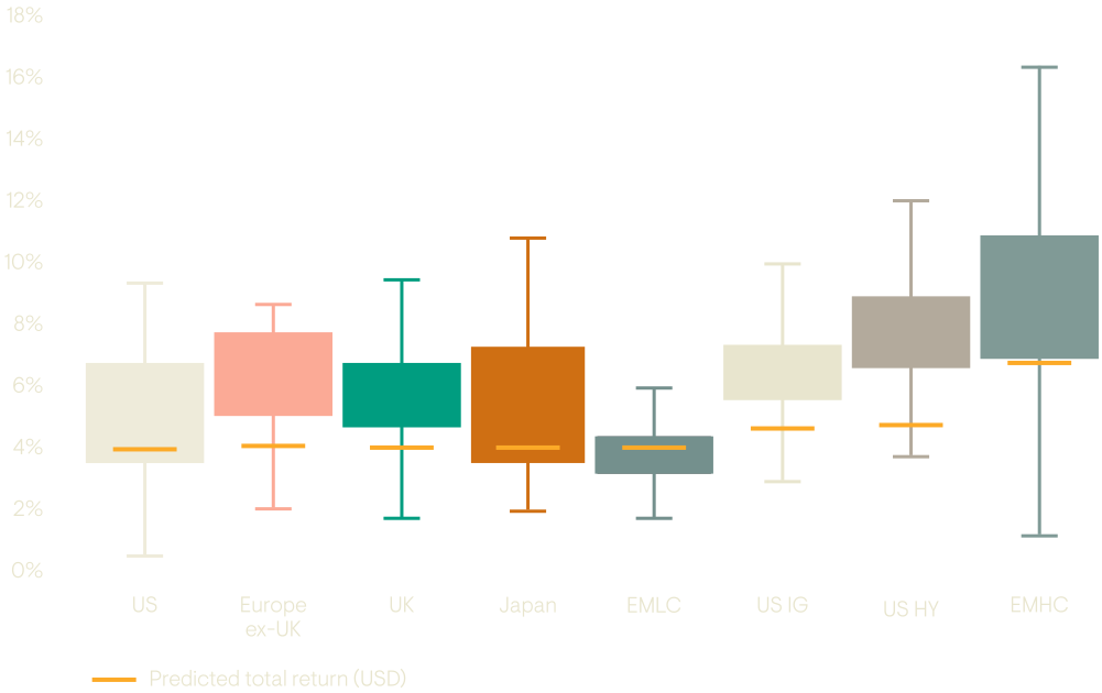
To better understand the relative attractiveness of prospective returns across fixed income markets, it is helpful to consider our return forecasts in the context of each market’s historic range of outcomes.

Figure 4: Historic returns

Source: Ninety One proprietary Capital Market Assumptions as at 31 March 2024. Estimates are nominal, hedged into USD, gross of fees and ignore alpha. Modelling involves risks, assumptions and uncertainties. These estimates reflect the view of Ninety One’s multi-asset team, while the views of other teams across Ninety One may differ. Performance does not guarantee future results. Actual returns could be materially higher or lower than projected. For information on our Capital Markets Assumptions methodology, please see Important information.
EMLC = Emerging Market Local Currency; EMHC = Emerging Market Hard Currency; US HY = US High Yield; US IG = US Investment Grade.

• The chart above shows the distribution of historic 10-year rolling geometric returns, hedged into USD, for the assets represented in the box-and-whisker plot, alongside the current forecast (yellow bar).
• The body of the box represents the interquartile range, while the ‘whiskers’ extend to the maximum and minimum historic rolling 10-year returns.
• It is evident that, apart from EMLC (in the second quartile), Japanese government bonds (roughly median) and US government bonds (just above the lower-quartile cut-off), expected fixed income returns are predicted to remain consistently in their lowest quartile.

Prospective global equity returns have remained relatively stable over the last six months, although regional movements have been varied. Within developed markets, the UK offers higher expected returns than other developed regions, while emerging markets only offer a modest return uplift relative to developed markets.

Figure 5: Equity: 10 year local currency return forecast

Performance does not guarantee future results. Actual returns could be materially higher or lower than projected.

Source: Ninety One (internal calculations based on Bloomberg data).

Prospective returns in Europe ex-UK and Japan have increased due to slight upward adjustments across the income, growth and revaluation drivers. In contrast, a dramatic rally in the Chinese equity market in late September has significantly reduced prospective returns in both China and emerging markets with negative revaluation returns now expected from both markets. Along with slightly lower income and trend growth estimates, the overall return forecast for China has notably decreased.

Expected returns from global equities remain disappointing, with the current forecast ranking among the lowest 10-year rolling outcomes of the last few decades.

Figure 6: Growth dominates return expectations, with revaluation almost uniformly negative

Performance does not guarantee future results. Actual returns could be materially higher or lower than projected.

Source: Ninety One (internal calculations based on Bloomberg data). Estimates are nominal, gross of fees and ignore alpha. The final total returns are converted from logarithmic to geometric estimates. This means that the components of the return breakdown may not sum to the total return. Judgmental overrides may apply where deemed necessary – for example as currently applied to the UK assumption to account for the region’s current dividend yield which is in our view structurally out-of-kilter both with its own history, and that of peers. Modelling involves risks, assumptions and uncertainties. These estimates reflect the view of Ninety One’s Multi-Asset team, while the views of other teams across Ninety One may differ.
For information on our Capital Markets Assumptions methodology, please see Important information. Return breakdowns in local currency.

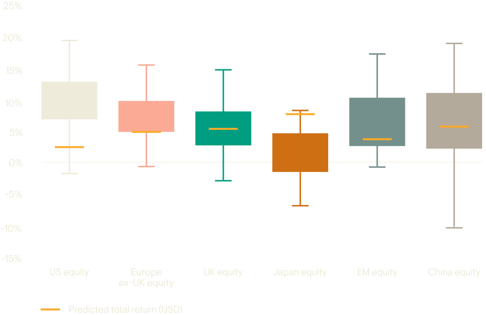
To better understand the relative attractiveness of prospective returns across equity markets, it is helpful to consider our return forecasts within the context of each market’s historical range of outcomes.

Figure 7: Historic returns

Source: Ninety One proprietary Capital Market Assumptions as at 30 September 2024. Estimates are nominal, hedged into USD, gross of fees and ignore alpha. Modelling involves risks, assumptions and uncertainties. These estimates reflect the view of Ninety One’s multi-asset team, while the views of other teams across Ninety One may differ. Performance does not guarantee future results. Actual returns could be materially higher or lower than projected. For information on our Capital Markets Assumptions methodology, please see Important information.

• The chart above shows the distribution of historic 10-year rolling geometric returns, hedged into USD, for the assets represented in the box-and-whisker plot, alongside the current forecast (yellow bar).
• The body of the box represents the interquartile range, while the ‘whiskers’ extend to the maximum and minimum historic rolling 10-year returns.
• While forecast equity returns generally appear unattractive in absolute terms, the US is comfortably in the lowest quartile compared to its recent history, with Europe ex-UK straddling lower-quartile returns. Japan, on the other hand, stands out with expected returns in the upper quartile of its recent history.

Over the last two years, investors have faced significant uncertainty over monetary policy, economic growth, inflation and geopolitics, leading to several waves of volatility in financial markets. Throughout this period, one constant has emerged: the outperformance of the largest US technology companies, collectively known as the Magnificent Seven². Since the start of 2023, an investment in the Magnificent Seven has tripled in value, while the US equity market (excluding these stocks) and the Global Equity ex-US market have each risen by about one third³. The dominance of these companies has been remarkable, as they now account for more than 30% of the S&P 500 index and almost 20% of the MSCI AC World index.

This has been a uniquely challenging environment for active equity investors, with limited avenues for outperformance beyond overweighting this narrow group of stocks. Moreover, the size of allocations to this handful of companies has disproportionately impacted the returns of even broadly diversified portfolios.

It certainly seems that the global equity market has been unusually concentrated during this period. More generally, a concentrated market can be characterised by returns that are tied to a small number of drivers – be it stocks, sectors, countries or factors.

We can also address the question of concentration from a more fundamental perspective by analysing market share within individual industries or the overall concentration of assets, revenues or profits across the market. This type of concentration raises broader questions about competition policy and how to foster innovation and productivity while ensuring outcomes that benefit consumers and the broader economy⁴.

How concentrated are equity markets relative to history?

To fully contextualise the current situation, we focus on US stock-level concentration, as this provides the longest data set for a broadly diversified equity market⁵. Although shorter- term data for the rest of the world is more limited, it suggests that the lessons derived may be generalisable.

Over the long run, the number of listed companies has trended higher, making it inappropriate to focus on a fixed number of stocks. Instead we look at the composition of the US equity market, broken down into deciles by market capitalisation.

This suggests that concentration within the US equity market is at or near historic extremes based on two distinct metrics:

• Market capitalisation of the largest decile: The market cap of the largest decile of stocks is more than 50 times that of the median US company. This ratio is comparable to the previous peaks in 1932 and 2000 and aligns with the well-documented outperformance of the largest US companies in recent years.
• Market capitalisation of the smallest decile: The market cap of the median company is 40 times that of the smallest decile. Relative to history, this is an even more pronounced outlier and exceeds the previous peak in 1991. There also appears to be a longer-term trend, dating back to the mid-20th century, of the smallest companies getting progressively smaller. This aspect of concentration is less frequently discussed but may be particularly interesting for active managers, especially those whose liquidity constraints allow them to explore opportunities in the bottom half of the market capitalisation distribution.

Figure 8: The average weight of the largest (top-decile) stocks has increased markedly vs. that of the median stock (coral)– which itself is much larger than historically the case vs. the smallest (bottom-decile) stocks (green)

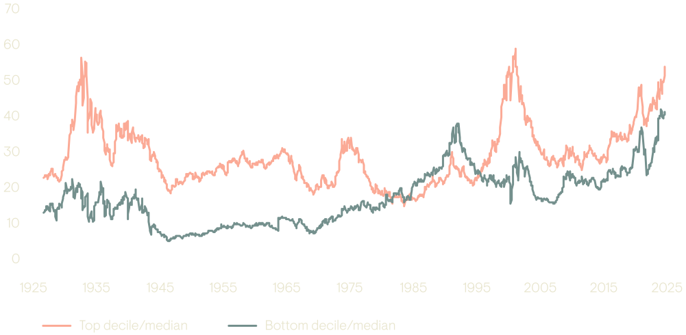
Source: Fama-French.

We can also assess concentration from a sector perspective. While the Magnificent Seven have distinct business models and span six different GICS industries, they can broadly be described as technology platform companies. Looking at sector weights over the long term, the rise of the technology sector is striking. Today, technology accounts for 40% of the overall US equity market, a share even greater than at the peak of the tech bubble in 2000.

Figure 9: The aggregate information technology sector weight is higher than at any time in the past century

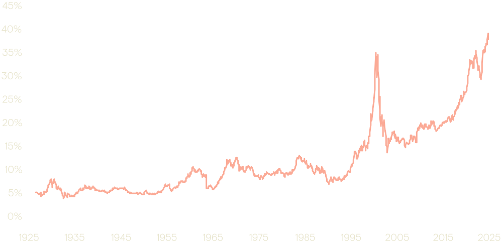
Source: Fama-French.

It appears that sector concentration may be even more pronounced than stock concentration. However, one could argue this simply reflects the evolution of technological progress or perhaps a failure to update sector definitions. Today, information technology is more integral and far-reaching than ever before.

Indeed, as Dimson, Marsh & Staunton show in Triumph of the Optimists, the major technology of the day always tends to dominate – for example, in 1900, railroads comprised 50% of the UK market and over 60% of the US market.

Figure 10: Sectors using industry classification from end-1899

Source: Triumph of the Optimists. Elroy Dimson, Paul Marsh & Mike Staunton.

What does history tell us about the relationship between concentration and returns?

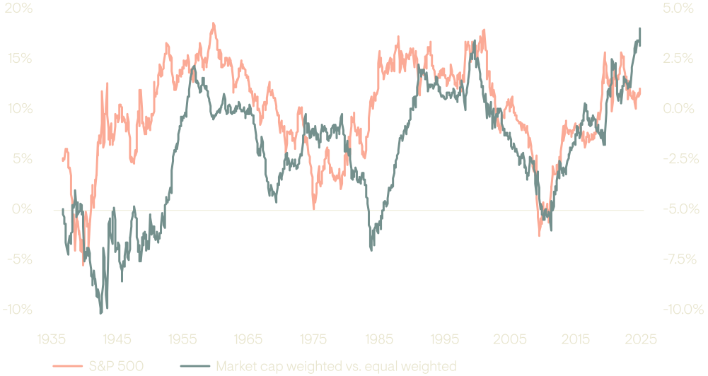
By definition, increasing concentration signals the relative outperformance of the largest companies – they grow even larger by outperforming the broader market. Notably, the substantial weight of these top index constituents significantly influences overall market returns, establishing a strong correlation between large-cap performance and the broader equity market’s direction. On a rolling 10-year basis, the recent outperformance of the largest US companies rivals any period in the past century, reflecting the robust market returns seen in this time.

Figure 11: Overall market performance (coral) is correlated with the outperformance of the cap-weighted vs. equally-weighted index (a proxy for large cap outperformance, green)

Source: Fama-French, Shiller.

While increasing concentration has been positive for overall market returns, it is likely that it has contributed to a difficult environment for active management. There are two primary mechanisms at play. Firstly, the scope for a skilled manager to outperform the market depends on skill being applied across a broad set of independent active risk positions. Given that outperformance has been concentrated in a small number of stocks and these stocks share many similar characteristics, the breadth opportunity has been more limited.

Secondly, further impacting breadth is the fact that overweight positions in large index constituents require allocating disproportionate amounts of capital to achieve the same active position size. For a US equity portfolio seeking to outperform the S&P 500 index, taking a 2% active position in Apple, currently the largest index constituent, would require a capital allocation of ~9.5%, taking the place of up to five similarly sized active positions in smaller index constituents.

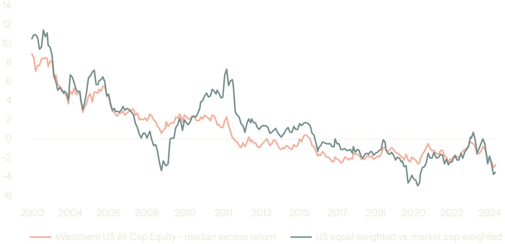
Historic performance of actively managed US equity portfolios also displays a clear link with the relative performance of the largest index constituents⁶. The chart below shows the excess returns of the median portfolio in the eVestment US All Cap Equity universe on a three year rolling basis. These returns closely match the relative performance of the MSCI USA equity weighted index relative to the MSCI USA market cap weighted index. The only period where the series diverge notably relates to the extreme market movements during the global financial crisis of 2008/9.

For a fuller discussion on the topic, see our forthcoming work on active management.

Figure 12: Concentration vs. active returns
Rolling 3 year returns

Source: eVestment, Bloomberg, MSCI.

Given today’s elevated concentration issues, it is natural to ask whether there are any implications for future returns.

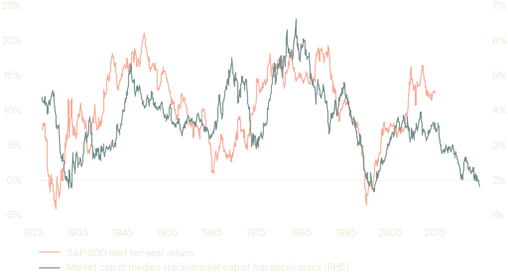
Here the historical data suggests a loosely defined but distinctly negative relationship, with high concentration associated with below-average future returns.

Figure 13: Forward market performance (coral) is loosely (inversely) correlated with the degree of market concentration (green) – the less concentrated the market, the better the forward returns historically

Source: Fama-French, Shiller.

This historic correlation may well be spurious as there doesn’t seem to be an inherent reason for it to hold; it’s unclear if there is an optimal level of concentration over time or across different industries.

Using our CMA framework, which breaks returns into income, growth and valuation components, we can examine the drivers of returns in a market with such extreme concentration and tease out the implications.

Income

Income is unlikely to significantly differentiate returns between high and low concentration markets. Although current income is low relative to long-term averages, this is not directly linked to market concentration.

Growth

Dividend growth has been a key driver of concentration, with the largest companies experiencing stronger growth than the rest of the market. Over the last decade, the aggregate revenues of the Magnificent Seven have grown by 16% per year, compared to just 6% for the average S&P 500 company. If this growth differential were to persist, it would likely support high future returns and potentially increase market concentration further.

Market composition impacts also appear favourable for returns in a concentrated market. In recent years, growing concentration has been accompanied by reduced negative impacts from market composition, as new entrants have struggled to challenge the dominance of the large incumbents. These companies, with substantial profits, have effectively utilised equity buybacks. Over the past decade, negative net issuance has been a positive driver of returns for the market-cap-weighted US equity market, adding 0.7% per annum to returns. By contrast, the equal weighted index experienced a negative impact of -2.1% per annum. Looking ahead, increased competitive intensity and higher capital expenditures from the largest companies could help to close this gap somewhat.

Valuation

Valuation has also been a key driver of concentration, as the largest companies have seen their valuations rise relative to the broader market, even after accounting for superior growth. While this trend can persist in the short term, history strongly suggests that in the long run, valuation reversion is a powerful driver of returns across equity markets. The starting point of high valuations in a concentrated market is likely to pose a headwind to US and global equity returns over a 10-year forecast horizon.

Do we need to adjust our CMA approach to deal with concentration?

Our current equity forecasts align with the muted return expectations historically associated with high market concentration, where elevated concentration often correlates with low future returns.

Examining the effectiveness of our forecasts historically, the only recent comparable scenario to today’s US equity market concentration is the tech bubble. When concentration peaked in December 2000, our process would have accurately identified a muted return outlook, with a forecast of just 0.5% per annum. The actual outcome over the subsequent decade was only slightly higher, at 0.9% per annum.

We don’t believe that overrides to our growth forecasts are necessary, as our approach relies on historic trend growth rates that evolve over time, reflecting any sustained shifts. This 10-year horizon approach helps avoid overreaction to short-term fluctuations. Although certain sectors may experience super-normal growth, such growth often attracts new competition, which drives rates back toward the average – though these averages levels may themselves increase over time, in line with Amara’s Law (“We tend to overestimate the effect of a technology in the short run and underestimate the effect in the long run”).

Equally, we see no need to adjust our valuation approach based on market concentration. Our process reflects current market composition and is capitalisation-weighted, with an underlying assumption that valuations eventually revert to long-term averages.

What’s particularly interesting today is the valuation disparity between the largest companies and the broader market. This suggests a plausible scenario where smaller companies could deliver significantly different returns compared to their larger peers. At the index level, returns would still be driven predominantly by the largest index constituents. However, for investors less tethered to index weights, the valuations of smaller companies appear to be much less of a headwind for returns.

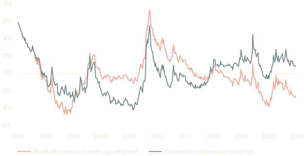
While we don’t produce forecasts for different market capitalisation segments, applying our valuation approach to both the market-cap weighted and equal-weighted versions of the MSCI USA index shows a valuation gap more pronounced than at any time in the last three decades.

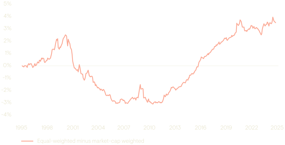
This can be seen in the chart below, which compares the revaluation return of the market-cap-weighted index (coral line, representing larger cap names) to that of the equally weighted index (green line, reflecting a greater focus on small- and mid-cap stocks). Additionally, we plot the difference between these two revaluation returns, providing a proxy for the relative outperformance of small and mid-cap stocks versus large caps.

This analysis shows that the equally weighted index has generally trended lower compared to the market cap weighted index, suggesting a devaluation trend. The expected return differential arising from revaluation alone currently stands at about 3.5% p.a. over the next decade. This mainly reflects the higher valuations of large-cap stocks (green line), while small- and mid-cap stocks (coral line), are more fairly priced.

Figure 14: Market-cap weighted US equity index is expected to experience significant negative impact from revaluation while the equal-weighted index sees a small positive impact. Valuation gap between largest companies and the rest of the market is the widest in 30 years.

Source: Ninety One (internal calculations based on Bloomberg data).

Conclusion

Equity market concentration is currently near historic highs, with the largest companies dominating both market cap and historic returns. Over the long-term, this level of concentration seems unsustainable. As a result, we believe it is reasonable to expect a general tapering-off of market returns, in line with historic trends and our current Capital Market Assumptions. Additionally, we expect market leadership to broaden as super-normal returns attract new entrants and regulators work to enforce and update competition policy. The relative valuation advantage of smaller companies points to an improved opportunity set for stock-selection, with increased potential for skill to be rewarded across a broader array of independent stock decisions.

² Apple, Microsoft, NVIDIA, Alphabet, Amazon, Meta & Tesla.
³ Source: Bloomberg. From 31 December 2022 to 30 September 2023, a market cap weighted investment in the Magnificent 7 returned 199%, the S&P 500 index excluding the Magnificent 7 returned 35% and the MSCI AC World index ex-USA returned 32%. All total returns in US dollars.
⁴ This is an area of active debate in academic and public policy settings. To give just one current example, Philippon et al have shown that regulatory approaches in the EU and the US have driven divergent outcomes in concentration in key sectors with European consumers benefitting from lower prices for mobile phones, home broadband, air travel and more. But Mario Draghi’s recent report for the EU Commission - The future of European competitiveness - further demonstrated that these more fragmented European industries with lower costs for consumers have limited the ability of companies to invest for the future and are a contributing factor to Europe falling behind the US in innovation and productivity growth.
⁵ Market concentration data has been collated for other markets over similarly long periods by Dimson, Marsh and Staunton for example but no other country comes close to the US in terms of breadth or global significance throughout the full period. Concentration metrics within smaller markets are liable to give a distorted picture. There are of course individual countries with extremely concentrated equity markets at times where a large global business is listed in a relatively small market – Novo Nordisk and TSMC currently represent over ¾ of the market in Denmark and Taiwan respectively.
⁶ Collecting representative data for the performance of actively managed portfolios is non-trivial and requires care to avoid self-selection and survivorship biases amongst other issues. There is no complete data set of all actively managed portfolios but eVestment appears to offer one of the best samples available. The data has very broad coverage of institutional portfolios and the process is well designed to exclude simulated or back-filled performance and maintains historic data for closed portfolios.

While we calculate our expected returns on a ̒local currency’ basis, we appreciate that clients need to make a currency decision – whether to hedge or not. To facilitate this, we present each of our equity and fixed income assumptions on two bases – hedged (using interest rate parity) and unhedged/converted (based on real exchange rate reversion).

Figure 15 Equity expectations

Source: Ninety One (internal calculations based on Bloomberg data).

Figure 16: Fixed income expectations

Source: Ninety One (internal calculations based on Bloomberg data).
EMBI = Emerging Markets Bond Index; EMLC = Emerging Market Local Currency; CEMBI = Corporate Emerging Markets Bond Index; US HY = US High Yield; US IG = US Investment Grade

Predicting long-term returns is fraught with difficulty; market values are not only determined by fundamentals, but also sentiment and exogenous events. We aim to keep things as straightforward as possible, and therefore focus on fundamentals. We:

We divide returns into three components. The first is known, more readily measured and widely available in the public domain, but the other two are subject to material misestimation:

By default, we assume a 10-year investment horizon, to reflect the fact that we are long-term stewards of client capital. We do not consider tax, given different requirements pertaining to different mandates. The approach we outline is our baseline estimate; we may make judgmental adjustments to the underlying drivers if warranted.

Our approach mimics that of a systematic investor, buying the entire market.

Here we set out our methodology for equities, fixed income and currencies:

⁷ Where a market has a high proportion of overseas sales, we use the average of the local and global nominal GDP per capita trend growth rates.
⁸ Uses the average of local and global issuance trends given lower predictability for more specific universes and a belief in global convergence. Overrides may also be applied where local figures are volatile.
⁹ Yield to Maturity based on notional 10-year bonds (except in the case of High Yield and EM Corporate, where 5-year bonds are used). For EM Hard Currency, US High Yield and EM Corporate, we use the underlying risk-free curve plus spread-to-worst to construct the initial yield.
¹⁰ Credit spread curve data tends to be unreliable; we presume because the notion of quality changes with tenor. We therefore assume a constant spread.
¹¹ This is an implicit allowance for rebalancing of the constant maturity bond.
¹² Based on Moody’s default data.

Equities

Equities are assumed to be purchased on a buy-and-hold basis. We use relevant MSCI indices to reflect the regions.

We proxy income with dividends. While many equity investors prefer to focus on earnings, we regard dividends as being less subject to manipulation – these distributions are a tangible payment, and the information is publicly disclosed – and therefore more reflective of the long-term fundamental cash-generating properties of the broad market. While other metrics (e.g. free cash flow) have evolved, they do not yet have similarly long history.

Figure 17: The history of US dividends stretches back over a century

Source: Shiller, U.S. Stock Markets 1871-Present and CAPE Ratio.

In this context, growth primarily relates to an equity market’s ability to increase dividends over time. GDP per capita has historically proven to be a reasonable proxy for dividend growth – and a closer match than GDP itself, as illustrated in the next chart. We simply allow for the global effects of growth based on the extent of non-domestic revenue exposure, assuming developed market growth is an average of local and global growth, while emerging market growth is wholly determined locally¹³. Growth is proxied based on trailing 15-year trend growth, a period that captures the secular effects of a couple of cycles. We apply a market adjustment factor – which includes changes in market composition relating to primary and secondary issuance, M&A activity, buybacks, new index inclusions etc. In each case, an owner of the market would have to either inject or remove capital to remain fully invested.

Figure 18: Nominal GDP per capita has proved a useful proxy for dividend growth

Source: Shiller, U.S. Stock Markets 1871-Present and CAPE Ratio; Samuel H. Williamson, “What was the US GDP Then?” MeasuringWorth, 2022.

Lastly, we factor in an adjustment for revaluation. We believe that valuation acts as a gravitational pull over long periods; however, changes in market composition and dynamic means that this is not a static metric. We use the price-dividend ratio and trend dividend yield as our valuation metric, assuming this reverts to a long-term (15-year) average. This allows us to both maintain consistency with our income-focused framework, and smooth out the cyclical nature of dividends. While we acknowledge full reversion is unlikely – prices tend to overshoot both on the upside and the downside – this simplification remains conceptually sound on average, as can be seen in Figure 19.

Figure 19: The actual price-dividend reverts reasonably neatly to the trend average over time

Source: Shiller, U.S. Stock Markets 1871-Present and CAPE Ratio, internal calculations.

Fixed Income

Our portfolios target specific duration contributions when allocating to bonds; therefore, we feel it appropriate to use constant maturity bonds as the basic building block. We further deconstruct bonds into risk-free and spread components, enabling us to cover both sovereign and corporate debt.

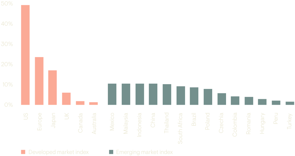
Income assumes the par yield of the bonds, typically for a notional 10-year bond. Regional indices are then generated by using the weighted average of the relevant market inclusions, as illustrated below.

Figure 20: Regional indices are generated using a weighted average of the relevant countries

Source: Ninety One calculations. Weights based on JP Morgan indices.

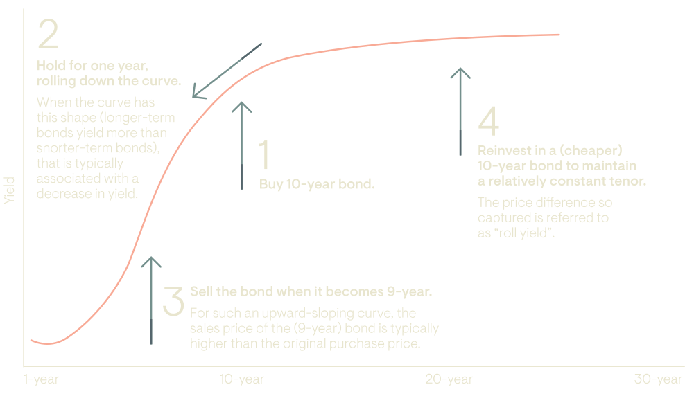
We define growth as being the roll yield obtained from consistently rebalancing the portfolio to maintain a constant maturity. So, for example, with a typical contango yield curve where the longer-term price is higher than the short-term, after one year the bond holder would sell the lower yielding, higher priced nine-year bond to buy a higher yielding, lower priced 10-year bond. Implicit in this view is a belief that the shape of the yield curve remains relatively consistent (including a constant spread component for credits).

Figure 21: Growth is the roll yield from consistently rebalancing the portfolio to maintain a constant maturity

Q In equities, why have you used GDP per capita and not GDP itself?

GDP per capita has historically proven to be a reasonable proxy for dividend growth.
This is even though the relationship between fundamental company growth, in aggregate, and country-level economic growth is weaker than might otherwise be expected due to compositional mismatches. For example, GDP includes both private and public sector outputs; however, only the former are captured in aggregate via listed equities. Similarly, economic growth tends to be locally focused whereas listed companies often have substantial global operations.

Q What assumptions do you make for credit defaults?

We make allowances for credit defaults with the bond growth rate, using Moody’s long-term default histories. We use the Moody’s country rating for specific country sovereign debt, and the ratings banding for credit indices. By assuming that a AAA rating has similar meaning in both sovereign and corporate contexts, we can reasonably proxy a wide array of indices. (Based on history, we have applied an additional default factor for sub investment grade sovereign debt).

Q Why nominal (and not real) returns?

Inflation is notoriously difficult to predict; so much so, that our work suggested that nominal forecasts were often more reliable than real forecasts.

Q Why two currency bases – hedged and converted?

Both are common approaches to international exposure – some prefer hedging, whereas others are prepared to bear the resultant currency risk. We therefore thought it appropriate to include both so, irrespective of preference, the assumptions would be useful.

Q How are Capital Market Assumptions used within the Multi-Asset process?

Capital Market Assumptions are a framework for thinking about reasonable client outcomes and providing broad market context. These figures do not directly result in individual investment decisions.

Importantly, the Capital Market Assumptions represent the view of the Multi-Asset Capability within Ninety One; other investment teams are free to disagree.

Q Are the assumptions purely systematic?

We wish the framework to be consistent over time to help sharpen thinking on asset-level drivers; therefore, where possible, we prefer to use set assumptions.

We do, however, reserve the right to override specific assumptions where there is a strong market-specific reason to do so.

Q Why do you not predict macro-economic variables within the Capital Market Assumptions?

We wish to understand potential client outcomes over the long-term; therefore, our focus is on identifying those drivers which best explain and predict such outcomes. As can be seen in our framework, that can be done without specific macro-economic views.

Q Why do your growth assumptions look so much more pessimistic than the last twenty years of equity and/or dividend growth?

For corporate cashflows to continue growing at a significantly faster rate than the broad economy, one of three things needs to occur:

• Revenue grows faster than the broad economy – e.g. via the launch of new products which are far superior to competitors, or through the capture of new market segments. The former should not make a difference at the aggregate market level (one competitors revenue growth comes at the expense of another) but the latter may occur through, for example, internationalisation. That is why we link growth to a mixture of local plus global GDP.
• Costs fall (or, equivalently, margins increase) – e.g. via lower tax rates, more efficient use of resources, economies of scale, or regulatory capture. We think further margin expansion is challenging as tax decreases have likely reached their nadir, while regulatory capture cannot happen indefinitely. Since we have not yet found a reasonable long-term (10-year) predictive proxy, we prefer not to forecast this element, i.e. assuming that margins remain roughly constant.
• Business reinvestment increases (when returns are higher than the cost of capital) – If businesses are prioritising their investment, marginal investments will offer a decreasing rate of return, such that ultimately returns converge to cost of capital. If not, we’d expect competitors to enter. Again, a natural limit exists. Again, in the absence of a reliable predictive proxy, we essentially assume that pay-out ratios remain constant.

In short – because we focus on variables that have both been historically predictive and have a sensible fundamental interpretation, we continue to favour GDP as a predictor (implicitly, of revenue). We continue to actively research appropriate variables for margins and pay-out ratios; however, in an environment where we think each faces headwinds, we are comfortable to continue with our simplifying assumption.

Q How often are your assumptions updated?

We intend to update the Capital Market Assumptions twice each year – after the March and September quarter-ends.

We may also provide intra-period updates if we believe a market event is significant enough to materially change the 10-year outlook. For example, we released an internal update in late March 2020 to highlight the potential upside from equities and credit after the initial COVID-induced market collapse.

Q What is an index divisor and what causes this value to change?

The index divisor is defined as:

Index divisor = Index market cap/Index price

The index divisor is central to the calculation of equity indices because there are corporate actions and compositional changes which affect the aggregate value or market capitalisation measured by the index, but which do not impact the performance of the index. When the market value of the index increases or decreases because of one of these events, the index divisor is adjusted to ensure that the price of the index remains unchanged.

The impact of specific corporate actions or compositional changes can be either positive or negative for future returns, but they are aggregated into a single overall value.

A non-exhaustive list of some of the corporate actions which impact the index divisor is given in the table below.

In addition, the composition of the index can change as a result of index rebalancing events where index rules determine that existing companies be added to or removed from an index or that the proportion of a company’s shares which are included in the index changes. For regional indices, whole countries may also be added or removed from the index.

Items such as buybacks tend to be stable – their attractiveness is based on the regulatory and taxation basis applicable at a point in time, which tend to change infrequently. Other sources may be more volatile – for example, market changes due to M&A activity, views on the appropriateness of stock-based compensation, or even secondary issuance due to market stress. We infer the market adjustment impact from the change in MSCI Index Divisor over time.

Q Have you considered the impact of issuance or other corporate activity on the growth of income within equities?

Broad economic growth drives the growth generated by the listed corporate sector over the long run. However, it is accepted that corporate action, including mergers, acquisitions, research, and innovation ensure that the corporate sector is dynamic, undergoing compositional changes over time.

Our process starts with an assessment of the aggregate growth of the dividends paid by this dynamic mix of businesses. The next step is to make a market adjustment to capture all the corporate actions and index composition changes which directly increase or decrease the total value of equity measured by the market index.

As defined, the market adjustment factor is important as it changes the participation in the aggregate dividend growth of the entire market for an ongoing investor in the index. Market adjustments at the index level are analogous to but not identical to the way that equity issuance and repurchases affect returns for a single stock. To understand this, we must first recognise that to receive the index return, an investor must build a portfolio which holds every stock in the index in their index weights and which adjusts these holdings over time as index composition and weights change.

Any corporate action or index composition change which adds new equity capital into the index therefore dilutes future index returns in the same way that a company making a rights issue dilutes returns for holders of that stock. In both cases, if an investor does nothing, their ownership of the index or of the stock declines and the proportion of future value creation which flows to their shares falls. On the flipside, any corporate action or index composition change which removes equity capital from the index is accretive to future returns in the same way that a company repurchasing and retiring existing shares is accretive.

Importantly, these effects only directly impact an investor who seeks to own the entire market as defined by the index provider. For an active investor who does not hold the companies which launch these corporate actions there is no direct impact on their returns although there may be indirect impacts because of related capital flows or changes in the competitive environment.

Q How effective have your Capital Market Assumptions been?

As can be seen in this analysis, the Capital Market Assumptions have shown clear differences between market troughs and market peaks.

Q Given that Capital Markets Assumptions have so much associated uncertainty, what is the benefit of even attempting?

We see two key benefits:

• A clear understanding of return drivers enables sharper thinking about potential asset class outcomes, including under various scenarios.
• Insight into the likely direction and possible magnitude of returns helps our clients understand what outcomes may be reasonable.

Q Why use dividends/price-dividend rather than earnings and the more conventional price/earnings?

Dividends, being physical payments to shareholders, are less subject to manipulation than earnings (which are only book profits). We believe that results in stronger conclusions.

In addition, data sets tend to have a longer history of dividend payments, enabling us to consider the approach in a broader variety of historic contexts.

Q What key factors are not considered in your approach?

Our Capital Market Assumptions assume that the fundamental market drivers remain unchanged. They therefore ignore exogenous shocks – e.g. climate risks and geopolitical events (although we may update our assumptions in the event of a material shock).

We currently focus on single-asset return outcomes; therefore, we make no comment about potential changes in cross-asset correlations or asset-specific volatilities.

We do not adjust for individual client circumstances either: client tax status may impact the relative attractiveness of asset classes.

Q Why a 10-year horizon?

As long-term custodians of our client’s capital, our focus is on helping our clients achieve suitable outcomes.

In addition, we require a timeframe long enough for fundamental drivers to be expressed, despite cyclical noise.