Latin America
Select your role
Capital Market Assumptions - April 2025
Ninety One’s Capital Market Assumptions framework focuses on the key drivers of long-term performance. We do this to better understand possible future returns, enriching discussions with our clients.
Apr 29, 2025
20 minutes
Ninety One’s Capital Market Assumptions framework focuses on the key drivers of long-term performance. We do this to better understand possible future returns, enriching discussions with our clients.
Our framework emphasises income payments across asset classes, as they are both readily measured and pivotal in determining returns. In addition, long-term history is available, and income is less subject to manipulation than accounting metrics.
We divide returns into three components. The first – income – is a tangible, known entity, but the others are subject to material misestimation:
| 1 | Income Yield is historically the single most important explanatory factor for income-generating assets |
| 2 | Growth The extent to which income is expected to change over time |
| 3 | Revaluation The price per unit of income likely to apply at the end of the period (typically, 10 years) |
Capital Market Assumptions - April 2025
Key takeaways

Major change is underway in the global economy. In domestic policy: the United States has undertaken to deregulate the economy, to shrink the Federal government and to bring down the pace of immigration; the European Union has shaken off self-imposed fiscal rules to dramatically increase investment in defence and infrastructure; and China has launched a ‘Special Action Plan’ to rebalance the economy through boosting domestic consumption. On the international front, the protectionist turn taken by the US has injected uncertainty into global production chains while hopes for peace in Ukraine and conflicts around the world have ebbed and flowed.
With so much going on, our Capital Market Assumptions offer an opportunity to take a step back and consider the longer-term outlook for global asset markets. We firmly believe a focus on the starting point (what you pay today) is crucial even when considering returns on a 10-year horizon. With elevated market volatility, it’s worth emphasising that this update is based on data as at 31 March 2025. The overall message is consistent with recent updates where we have presented a picture of low expected returns in aggregate. We anticipate that a traditional 60% global equity, 40% global government bond portfolio will deliver a 4.4% annualised return for the next decade in nominal terms, when hedged into US dollars. This represents a modest improvement in the forward-looking return opportunity, with an uplift across both equities and fixed income.
We continue to see a need for considerable value-add from asset allocation and security selection decisions as well as from identifying investments that will benefit from structural growth tailwinds to achieve investment objectives.
Forecasts are inherently limited and modelling involves risks, assumptions and uncertainties, they are forward looking and are not guarantees nor a reliable indicator of future results. Actual returns could be materially higher or lower than projected. This information is not intended as a recommendation to invest in any particular asset class or strategy or as a promise of future performance.
Source: Ninety One proprietary Capital Market Assumptions as at 31 March 2025. These estimates are gross of fees (returns can be reduced by management fees and other expenses incurred) and reflect the view of Ninety One’s multi-asset team, whilst the views of other teams across Ninety One may differ. Details on our Capital Market Assumptions methodology available upon request.
Capital Market Assumptions - April 2025
Key takeaways
The pace of change in the global economy has accelerated with major policy shifts in the US, Europe and China. We look through the noise and focus on the longer-term drivers of returns.
Major change is underway in the global economy. In domestic policy: the United States has undertaken to deregulate the economy, to shrink the Federal government and to bring down the pace of immigration; the European Union has shaken off self-imposed fiscal rules to dramatically increase investment in defence and infrastructure; and China has launched a ‘Special Action Plan’ to rebalance the economy through boosting domestic consumption. On the international front, the protectionist turn taken by the US has injected uncertainty into global production chains while hopes for peace in Ukraine and conflicts around the world have ebbed and flowed.
With so much going on, our Capital Market Assumptions offer an opportunity to take a step back and consider the longer-term outlook for global asset markets. We firmly believe a focus on the starting point (what you pay today) is crucial even when considering returns on a 10-year horizon. With elevated market volatility, it’s worth emphasising that this update is based on data as at 31 March 2025. The overall message is consistent with recent updates where we have presented a picture of low expected returns in aggregate. We anticipate that a traditional 60% global equity, 40% global government bond portfolio will deliver a 4.4% annualised return for the next decade in nominal terms, when hedged into US dollars. This represents a modest improvement in the forward-looking return opportunity, with an uplift across both equities and fixed income.
We continue to see a need for considerable value-add from asset allocation and security selection decisions as well as from identifying investments that will benefit from structural growth tailwinds to achieve investment objectives.
Forecasts are inherently limited and modelling involves risks, assumptions and uncertainties, they are forward looking and are not guarantees nor a reliable indicator of future results. Actual returns could be materially higher or lower than projected. This information is not intended as a recommendation to invest in any particular asset class or strategy or as a promise of future performance.
Source: Ninety One proprietary Capital Market Assumptions as at 31 March 2025. These estimates are gross of fees (returns can be reduced by management fees and other expenses incurred) and reflect the view of Ninety One’s multi-asset team, whilst the views of other teams across Ninety One may differ. Details on our Capital Market Assumptions methodology available upon request.
Historical effectiveness
We tend to evaluate effectiveness in terms of getting the direction of travel correct.
Long-term predictions are fraught with uncertainty and open to error. We can, however, retrospectively apply our framework to assess its historical effectiveness. Because we focus on contextual information, we tend to evaluate effectiveness in terms of the reliability of the direction of the signal at market peaks or troughs; getting the broad direction of travel correct over a decade is a critical factor in an overall investment outcome.
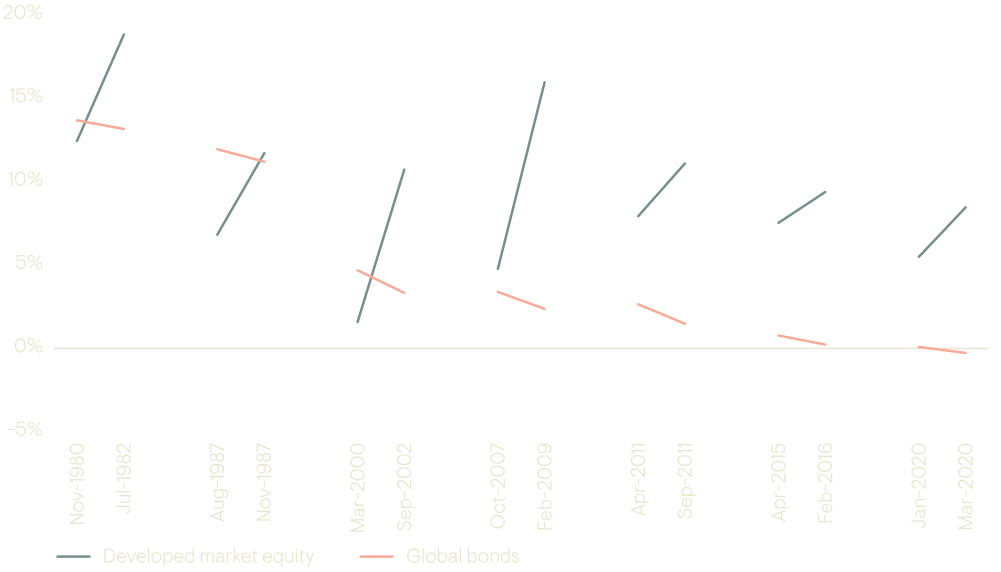
The figure below identifies a variety of market peaks and subsequent troughs, stretching back to 1980, for each of developed market equity and global bonds1. We then show the subsequent 10-year predicted returns at those points.
Figure 1: Expected returns can vary significantly depending on the point of the cycle
Source: Ninety One. Data is global since 2000; prior dates based on US outcomes. Bonds based on 10-year tenor.
For example, the first point on the previous chart corresponds to November 1980 (roughly a market peak) followed by a trough in July of 1982. The relevant 10-year forecasts in each instance were:
| Peak | Subsequent trough | |
|---|---|---|
| Developed market equity | 12.4% | 18.8% |
| Global bonds | 13.7% | 13.2% |
Indeed, global equities tripled in the decade from November 1980, and rose fourfold from July 1982. The chart illustrates the desired pattern — riskier assets tend to have lower anticipated 10-year returns at peak than they do at the subsequent trough; conversely, the more defensive bond asset tends to do better at the peak than the trough. Interestingly, although this pattern is repeated over time, it does appear to be getting more compressed – perhaps due to the expansive liquidity provision over this period.
1 Developed market equities = MSCI ACWI and global bonds = FTSE WGBI.
Fixed income
Prospective returns from global government bonds have risen slightly along with the additional compensation from taking on greater credit risk.
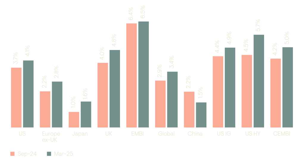
The following chart examines fixed income assets in nominal, local currency terms, for 31 March 2025 versus our last update, six months ago:
Figure 2: Sovereign bond yields and credit spreads have both increased modestly
10-year local currency, return forecast
Source: Ninety One (internal calculations based on Bloomberg, JP Morgan and Moody’s data). EMBI = Emerging Markets Bond Index, EM LC = Emerging markets local currency debt; US IG = US investment grade; US HY = US high yield; CEMBI = Corporate Emerging Markets Bond Index.
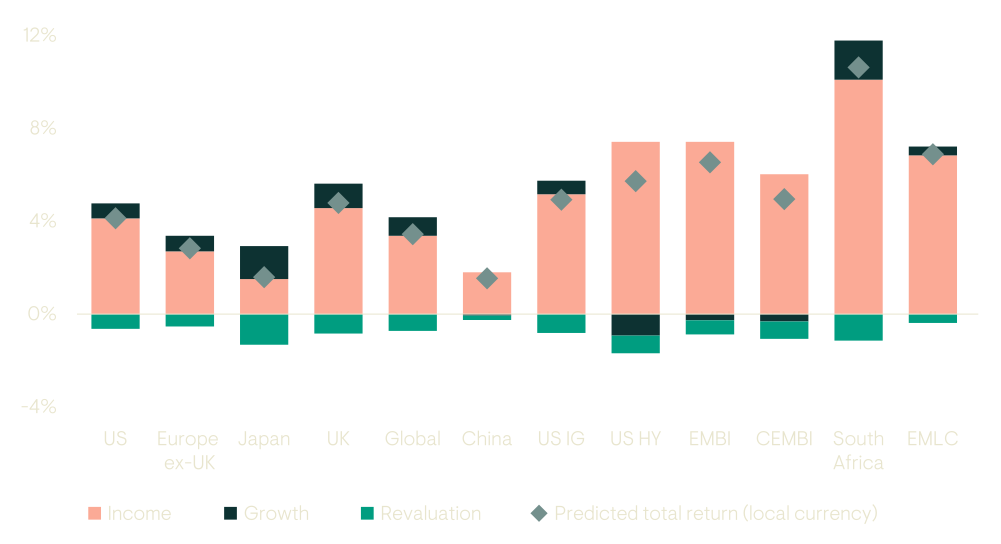
Most markets show an increase in prospective returns over the last six months, with income continuing to dominate returns. Credit spreads have increased slightly but remain very low in a historical context.
Risk-free yields remain consistently lower than those implicit in forward yield curves, leading to negative revaluation effects across the board. Monetary policy easing cycles remain in progress in most economies, with Japan and Brazil among the few exceptions that are continuing to raise official interest rates.
To illustrate the dynamic nature of our forecasts, we also estimate how our expectations were affected by market moves which occurred just after quarter-end. One of the most impacted assets was US high yield corporate bonds, where both US treasury yields and credit spreads moved higher.
At their peak on 8 April 2025, US high yield bond yields had risen by 100bps from their 31 March level, with spreads returning almost exactly to their 15-year average. This shift increased the income component of expected returns and removed the previously negative contribution from long-term spread mean reversion. At that point, our total return forecast for US high yield would have risen by 1.4% to 7.1% per annum (in log local currency terms).
The following chart sets out our return forecasts in more detail, dissecting fixed income regions in the context of our Capital Market Assumptions framework pillars: income, growth, and revaluation.
Figure 3: Income accounts for the bulk of return potential across fixed income
Source: Ninety One (internal calculations based on Bloomberg, JP Morgan and Moody’s data). US IG = US Investment Grade; US HY = US High Yield; EMBI = Emerging Markets Bond Index; CEMBI = Corporate Emerging Markets Bond Index; EMLC = Emerging Market Local Currency.
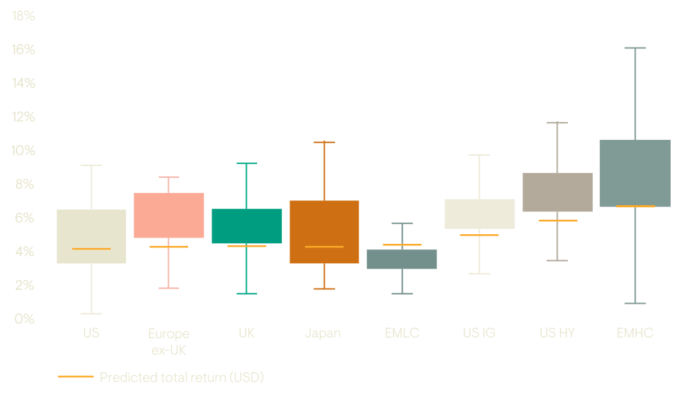
To give a further understanding of the relative attractiveness of prospective returns across fixed income markets, it is helpful to consider our return forecasts in the context of the historic range of outcomes for each market.
Figure 4: Return distribution of 10-year rolling historic returns
Source: Ninety One proprietary Capital Market Assumptions as at 31 March 2025. Based on monthly data from December 1987 to March 2025. Estimates are nominal, hedged into USD, gross of fees and ignore alpha. Modelling involves risks, assumptions and uncertainties. These estimates reflect the view of Ninety One’s multi-asset team, while the views of other teams across Ninety One may differ. Performance does not guarantee future results. Actual returns could be materially higher or lower than projected. For information on our Capital Markets Assumptions methodology, please see Important information. EMLC = Emerging Market Local Currency; EMHC = Emerging Market Hard Currency; US HY = US High Yield; US IG = US Investment Grade.
- The chart above shows the distribution of historic 10-year rolling geometric returns, hedged into USD, for the assets (in the box-and-whisker plot) versus the current forecast (yellow bar).
- The body of the box represents the interquartile range, while the ‘whiskers’ extend to the maximum and minimum historic rolling 10-year returns.
- It is evident that, bar EM LC (top quartile) and EM HC (second quartile), fixed income returns are predicted to be consistently below historic median returns.
Equities
Return expectations remain low but have moved up slightly. Prospective returns are somewhat higher in Japan, the UK and emerging markets relative to US and Europe ex-UK.
Prospective returns have increased across global developed and emerging markets, primarily as a result of a lower forecast drag from revaluation. This has occurred as aggregate global equity and global emerging market index prices were slightly lower over the period while our estimates of underlying trend dividends moved up. There was significant dispersion within equities over the period, reflected in slightly lower return forecasts for China, South Africa and the UK – the markets that delivered the strongest positive returns over the period.
The following chart shows forecasted returns for equity markets in nominal, local currency terms, as at 31 March 2025 versus our last update, six months ago.
Figure 5: Equity: 10 year local currency return forecast
Performance does not guarantee future results. Actual returns could be materially higher or lower than projected.
Source: Ninety One (internal calculations based on Bloomberg data).
Expected returns from global equities remain at the low end of 10-year rolling outcomes historically.
Figure 6: Growth dominates return expectations, with revaluation almost uniformly negative
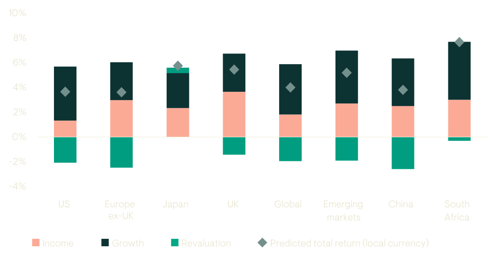
Performance does not guarantee future results. Actual returns could be materially higher or lower than projected.
Source: Ninety One (internal calculations based on Bloomberg data). Estimates are nominal, gross of fees and ignore alpha. The final total returns are converted from logarithmic to geometric estimates. This means that the components of the return breakdown may not sum to the total return. Judgmental overrides may apply where deemed necessary – for example as currently applied to the UK assumption to account for the region’s current dividend yield which is in our view structurally out-of-kilter both with its own history, and that of peers. Modelling involves risks, assumptions and uncertainties. These estimates reflect the view of Ninety One’s Multi-Asset team, while the views of other teams across Ninety One may differ.
For information on our Capital Markets Assumptions methodology, please see Important information. Return breakdowns in local currency.
To illustrate the dynamic nature of our forecasts, we can also estimate how our expectations were affected by the market drawdown immediately after quarter-end. At the closing low on 8 April 2025, global equities had declined by 10% from their 31 March level. At that point, the reduced drag from the revaluation component would have increased the global equity return forecast by 1.0%, bringing it to 5.0% per annum (in log local currency terms).
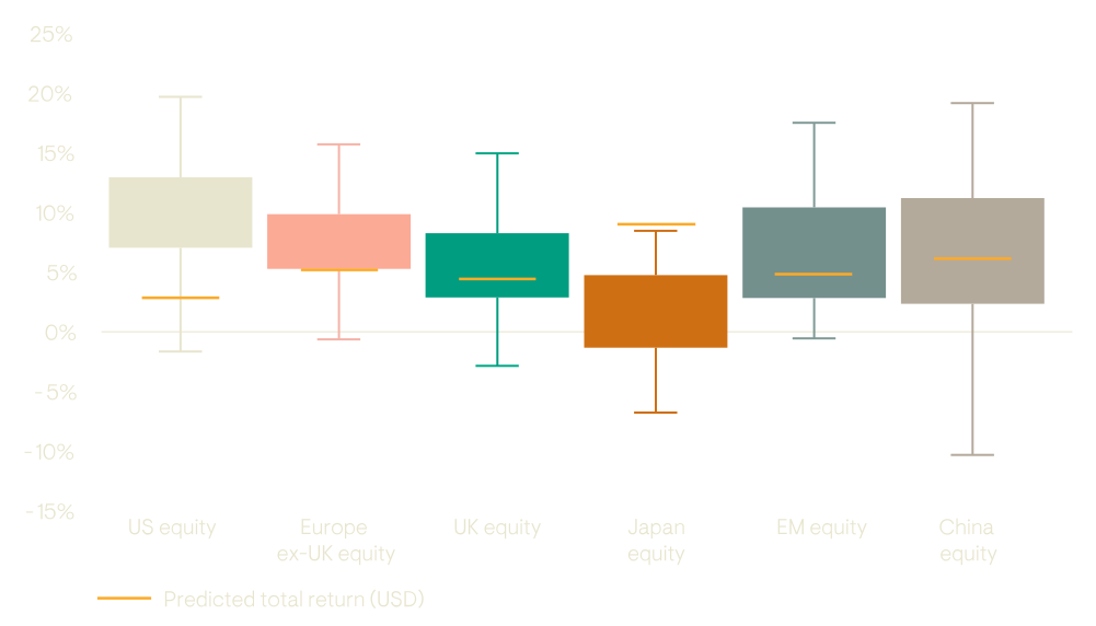
To give a further understanding of the relative attractiveness of prospective returns across equity markets, it is helpful to consider our return forecasts in the context of the historic range of outcomes for each market.
Figure 7: Return distribution of 10-year rolling historic returns
Source: Ninety One proprietary Capital Market Assumptions as at 31 March 2025. Based on monthly data from December 1987 to March 2025. Estimates are nominal, hedged into USD, gross of fees and ignore alpha. Modelling involves risks, assumptions and uncertainties. These estimates reflect the view of Ninety One’s multi-asset team, while the views of other teams across Ninety One may differ. Performance does not guarantee future results. Actual returns could be materially higher or lower than projected. For information on our Capital Markets Assumptions methodology, please see Important information.
- The chart above shows the distribution of historic 10-year rolling geometric returns, hedged into USD, for the assets (in the box-and-whisker plot) versus the current forecast (yellow bar).
- The body of the box represents the interquartile range, while the ‘whiskers’ extend to the maximum and minimum historic rolling 10-year returns.
- While forecast equity returns do not generally look attractive in an absolute sense, the US is comfortably in the lowest quartile versus its recent recent history, with Europe ex-UK straddling lower-quartile returns. Japan stands out on this basis, with expected returns in line with the maximum return in recent history.
Case study: US uniqueness or European exceptionalism?
US exceptionalism has become a recurring theme in economic and market commentary in recent years. The label stretches across a broad spectrum — from America’s dynamic business culture and capacity for innovation to the scale of government spending that has helped sustain growth and the US dollar’s outsized role in global finance.
In financial markets, the clearest expression of US exceptionalism has been the prolonged and significant outperformance of American equities over the past decade. Using the framework underpinning our capital market assumptions, we can break down the sources of equity market returns — helping us understand what has driven this outcome and what it might mean for US and other regional markets over the next ten years.
We begin by turning back the clock to consider how our framework would have viewed US return prospects before the era of exceptionalism took hold. From there, we deconstruct the drivers of equity returns to better understand what propelled US equities to the top of the global leaderboard.
This analysis also reveals that European equity performance has been exceptional — though in a very different sense. As major policy shifts take shape across the continent, investors are weighing the possibility of a structural change in Europe’s growth trajectory. In the final section, we place this potential inflection point in a historical context and consider the precedents for such transformations.
US exceptionalism in equity returns
For this analysis, we focus on the 10 years to 31 December 2024. This aligns with our forecast horizon and captures the period in which US equity outperformance was most pronounced.
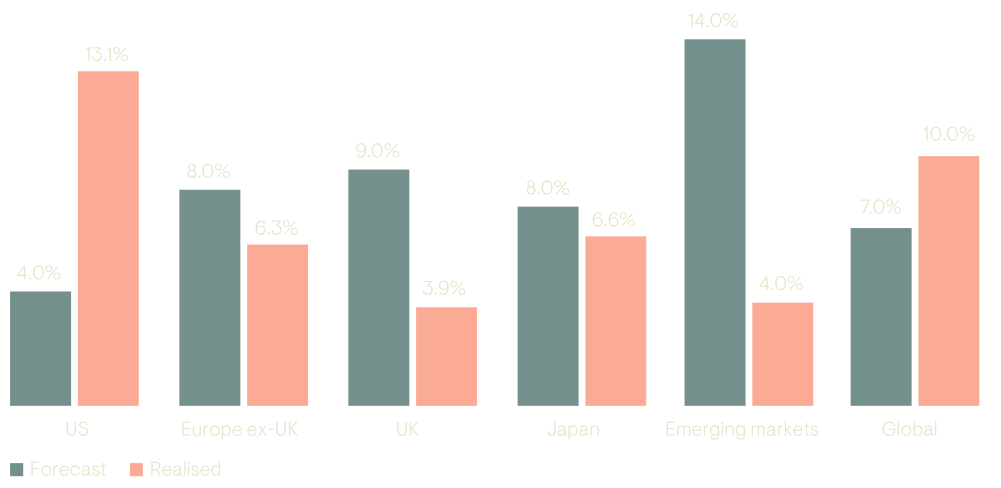
The first lens through which we assess US exceptionalism is a comparison between our CMA model forecasts for regional equity markets and the actual outcomes over the decade.
As shown in Figure 8, US equities far outpaced modelled expectations. The realised return of 13% p.a. was nearly three times the forecast return of 4.5% p.a. — a striking deviation not only from our projections but also from the long-run historical average. In the 100 years to 2014, US equities returned 7% p.a. With US equities making up over half the global market at the start of the period and approximately 2/3 at the end of the period, this underestimate for the US equity market also resulted in a (smaller) underestimate for the global equity market.
In contrast, the model’s forecasts for other regions proved consistently overoptimistic. While returns for European and Japanese equities fell within expected error bands, outcomes for the UK — and especially emerging markets — were notably weaker than anticipated.
Figure 8: Regional equity forecasts and realised returns, 10 years to 31 December 2024, USD converted terms
Source: Ninety One (internal calculations based on Bloomberg and MSCI data).
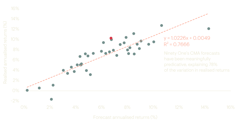
Forecasts for individual markets are subject to larger errors than forecasts for the global equity market given the scope for greater impact from idiosyncratic factors. When assessing the ability of our approach to capture information about the prospective returns available in equities, it makes most sense to focus on the global market. Looking back at the modelled outcomes based on information which would have been available at the time and comparing those to the actual outcomes, Figure 9 demonstrates a strong linear relationship with little suggestion of results being skewed towards either over- or under-optimism. The fact that there are notable errors in individual 10 year periods is to be expected given the high degree of uncertainty inherent in the exercise and the scope for markets to deviate from a consistent pricing of long-term fundamentals at times of excessive fear or greed.
Each dot in Figure 9 represents the period aligned to our 6-monthly update schedule with the red dot showing the 10-year period starting on 30 September 2014 or essentially the same period as that covered by this analysis of US exceptionalism. This period was the largest single underestimate in the historic data going back 30 years, which further underlines the uniqueness of this episode.2
Figure 9: 10-year forecast vs. actual equity returns — rolling periods from March 1995 to March 2015
10-year local currency, return forecast
Source: Ninety One (internal calculations based on Bloomberg and Moody’s data).
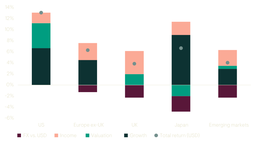
To understand how these outcomes diverged so sharply from expectations, we break down the actual outcomes in Figure 10. The US market saw by far the largest positive revaluation and second-highest growth in earnings after Japan. The scale of the valuation uplift change stands out: only the UK and emerging markets (EM) experienced modest gains, while valuations were flat in Europe ex-UK and declined in Japan.
The US dollar appreciated against all other regional currencies, amplifying the extent of US outperformance when measured in common currency terms without hedging. Equity and FX effects were closely intertwined — the strength of the US economy and equity market helped drive capital flows into the US, reinforcing demand for the dollar relative to other currencies.
Figure 10: Drivers of regional equity returns, 10 years to 31 December 2024, USD converted
Source: Ninety One (internal calculations based on Bloomberg and MSCI data).
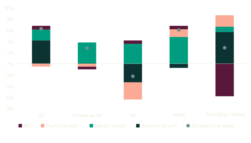
We can break dividend per share growth into four components: aggregate revenue growth, margin changes, payout ratio changes, and market composition impacts (MCI), as shown in Figure 11. The most striking divergence appears at the revenue line. US revenue growth was solid and broadly in line with expectations, but revenues were flat over the decade in Europe and declined outright in Japan and the UK. EM posted slightly higher revenue growth than the US, though as we have examined in more detail, this was offset by a larger-than-expected drag from market composition changes.
Margin expansion contributed positively across all regions and was, in fact, more significant in developed markets outside the US.
Figure 11: Drivers of growth, 10 years to 31 December 2024, local currency terms
Source: Ninety One (internal calculations based on Bloomberg and MSCI data).
US equity returns stand out for the extent to which they exceeded both our CMA forecasts and long-run historical benchmarks. The primary drivers of this outperformance were a substantial revaluation and a stronger US dollar, as global capital flowed into US equities. These were underpinned by solid fundamentals: US revenues, earnings and dividends grew faster than in other regions.
Importantly, US growth was not exceptional by historical standards. Rather, it was the relative weakness of other markets — especially the stagnation in developed market revenues outside the US — that made the US performance appear so dominant.
European growth prospects
The stagnation in European revenue growth over the past decade is exceptional — for all the wrong reasons. Alongside geopolitical pressures, it has fuelled a growing imperative for policymakers to shift the continent’s economic trajectory.
At a time of heightened uncertainty and with significant policy change, it is difficult to forecast how these efforts will translate into growth. What the CMA framework can offer is perspective: a long-term, data-driven context to ground expectations.
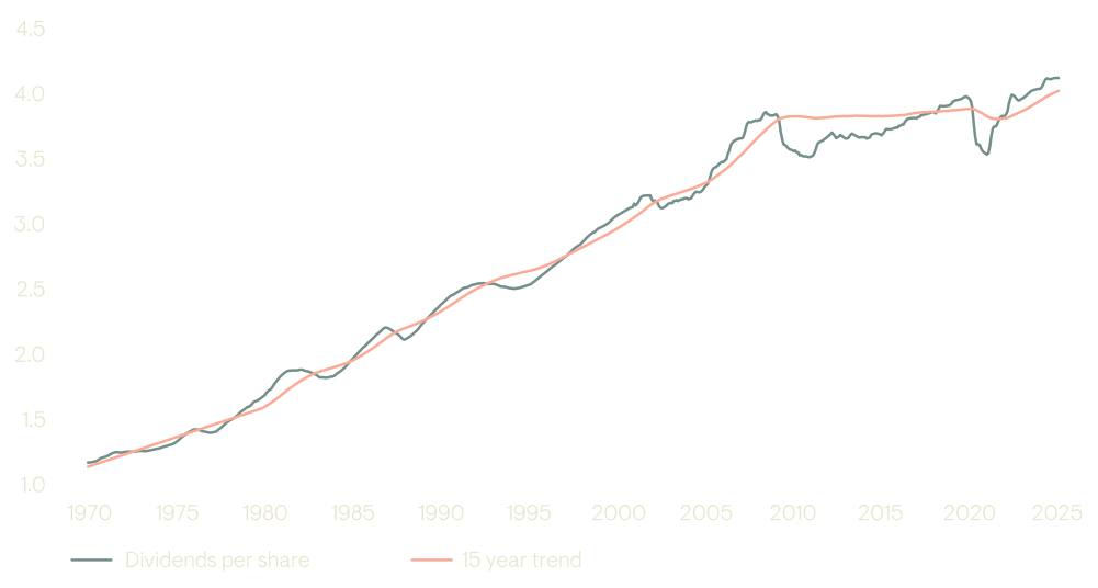
To this end, we look as far back as the data allows — tracking the progression of dividends over more than 50 years. This long view reveals just how unusual the post-GFC period has been. Since 2008, dividend growth in Europe has stalled. This stands in stark contrast to the previous four decades when dividend growth followed a remarkably steady, near-linear trend.
Figure 12 shows the trailing 12-month dividends per share for the MSCI Europe index in log terms. The 15-year trend measure used is the same one that underpins our CMA estimates of underlying dividend growth. On a log scale, the steady trend from 1970 to 2008 suggests a consistent growth rate in Europe’s dividend-paying capacity over that period.
If the factors suppressing growth post-GFC prove temporary, there may be scope for Europe to rejoin its historical trend — a return to a more normal growth environment.
Figure 12: MSCI Europe dividends per share (log scale)
Source: Ninety One (internal calculations based on MSCI data) as at 31 March 2025.
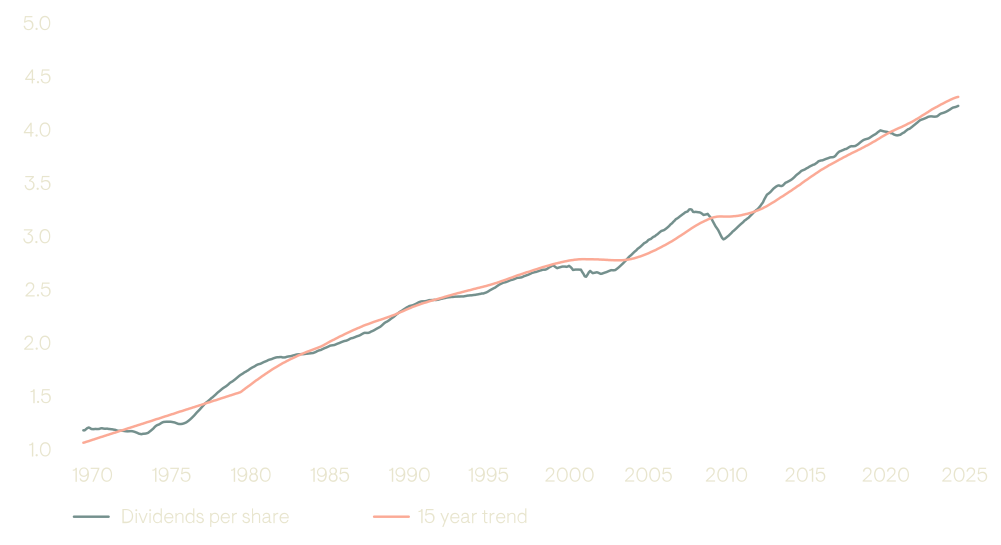
This long-term view also helps put the US experience in perspective. Figure 13 shows that the recent US growth outcome, while strong, is not historically unusual. The progression of trend dividends in the US market has followed a remarkably consistent path since 1970, reinforcing the idea that recent performance reflects continuity rather than a structural break.
Figure 13: MSCI USA dividends per share (log scale)
Source: Ninety One (internal calculations based on MSCI data) as at 31 March 2025.
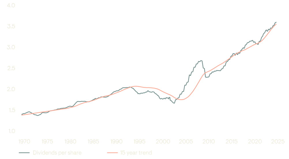
Japan, the other developed market with a long dividend history, offers a useful parallel to Europe. After its stock market and real estate collapse in the early 1990s, Japan entered a prolonged period of stagnation — dividends per share did not surpass their 1991 level until 2005. What followed, however, was a striking corporate renaissance. A combination of governance reforms, improved capital discipline, and stronger shareholder focus helped drive a sustained recovery. Dividend growth reaccelerated, and the long-run trend rose to a level well above that seen in the 1970s and 1980s.
Figure 14: MSCI Japan dividends per share (log scale)
Source: Ninety One (internal calculations based on MSCI data) as at 31 March 2025.
In conclusion, the US equity market was truly unique over the past decade — both in the scale of its re-rating and in its relative growth performance against a weak global backdrop. Our CMA forecasts point to a partial reversal of the valuation expansion and to dividend growth more in line with long-run trends in revenue and per capita GDP. If this plays out, the return profile for US equities is likely to be significantly lower over the next decade.
In contrast, the exceptional growth story — albeit of a different kind — was in Europe, where it took 15 years for dividends to recover sustainably above their pre-GFC peak. But both Europe’s longer-term history and Japan’s recovery from its own lost decade suggest that a return to moderate, through-the-cycle growth is a reasonable central case for European equities.
Taken together, our process points to similar return expectations for US and European equities over the coming decade — a potential period of convergence after an era of unusually wide divergence.
2 The largest absolute error by contrast was an overestimate for the period starting on 31 March 1999 where the model predicted a return of +2.1% but the actual outcome was -1.6% per annum.
Currency
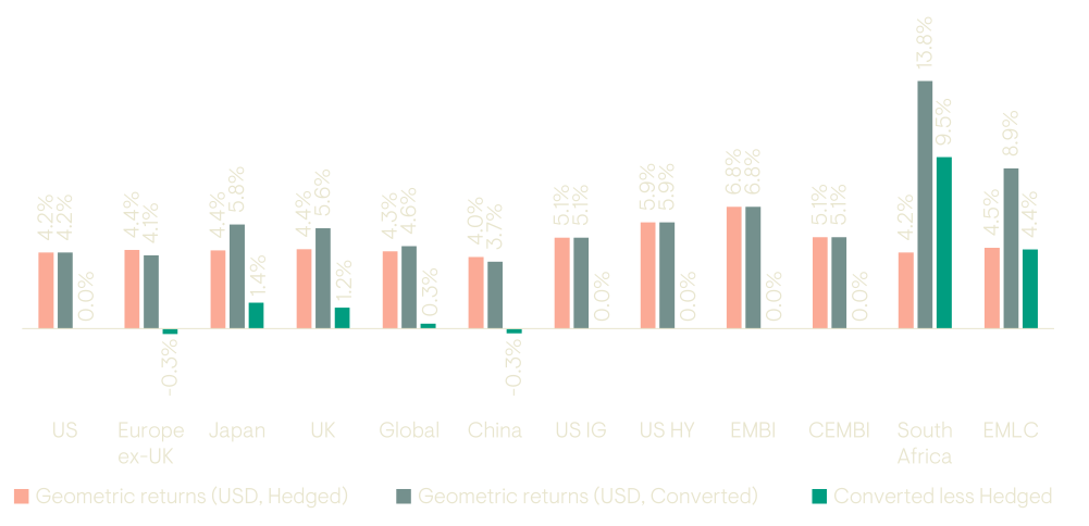
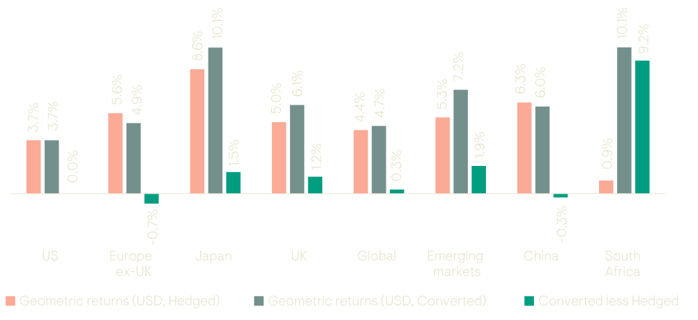
The currency decision – particularly whether to use ‘hedging’ or ‘conversion’ – can have a material impact on the outcome.
While we calculate our expected returns on a ̒local currency’ basis, we appreciate that clients need to make a currency decision – whether to hedge or not. We therefore show each of our equity and fixed income assumptions on these two bases – hedged (using interest rate parity) and unhedged/converted (based on real exchange rate reversion).
Figure 15: Fixed income expectations
Source: Ninety One (internal calculations based on Bloomberg and JP Morgan data). US IG = US Investment Grade; US HY = US High Yield; EMBI = Emerging Markets Bond Index; CEMBI = Corporate Emerging Markets Bond Index; EMLC = Emerging Market Local Currency.
Figure 16: Equity expectations
Source: Ninety One (internal calculations based on Bloomberg data).
Methodology
We focus on fundamentals. We divide returns into three components. The first is known and widely available, but the other two are subject to material misestimation.
Predicting long-term returns is fraught with difficulty; market values are not only determined by fundamentals, but also sentiment and exogenous events. We aim to keep things as straightforward as possible, and therefore focus on fundamentals. We:
|
Favour simplicity to capture the key drivers and accept wide uncertainty bands |
Strive for consistency with the investment process, focusing on cashflows |
Aim to be comprehensive across asset classes, with the ability to extend within |
We divide returns into three components. The first is known, more readily measured and widely available in the public domain, but the other two are subject to material misestimation:
|
Income – yield is the single most important explanatory factor for income-generating assets |
Growth – the extent to which income will likely change over time |
Revaluation – the price per unit of income likely to apply at the end of the period |
By default, we assume a 10-year investment horizon, to reflect the fact that we are long-term stewards of client capital. We do not consider tax, given different requirements pertaining to different mandates. The approach we outline is our baseline estimate; we may make judgmental adjustments to the underlying drivers if warranted.
Our approach mimics that of a systematic investor, buying the entire market.
Here we set out our methodology for equities, fixed income and currencies:
|
|
Equities |
Sovereign debt and credit |
|---|---|---|
|
Income |
Current dividend yield |
Current yield on notional bond5 |
|
Growth |
Nominal GDP per capita3 growth plus Market composition impacts (IPOs, M&A, index inclusion events etc)4 (Each based on a 15-year historic trend) |
Anticipated change in yield based on market-inferred future risk-free yields6 plus Roll-yield on the risk-free curve7 less Credit losses based on a 15-year historic average8 |
|
Revaluation |
Reversion to a cyclically adjusted price-to-dividend ratio (based on 15-year trend dividends per share) |
Reversion to the market-inferred future risk-free yields plus Reversion of credit spread to 15-year average |
|
Currency |
‘Hedging’ – based on current interest rate differentials on 10-year zero-coupon bonds or ‘Conversion’ – based on a reversion of the real exchange rate to the 15-year average, with an allowance for differences in inflation targets |
|
3 Where a market has a high proportion of overseas sales, we use the average of the local and global nominal GDP per capita trend growth rates.
4 Uses the average of local and global issuance trends given lower predictability for more specific universes and a belief in global convergence.
Overrides may also be applied where local figures are volatile.
5 Yield to Maturity based on notional 10-year bonds (except in the case of High Yield and EM Corporate, where 5-year bonds are used).
For EM Hard Currency, US High Yield and EM Corporate, we use the underlying risk-free curve plus spread-to-worst to construct the initial yield.
6 Credit spread curve data tends to be unreliable; we presume because the notion of quality changes with tenor. We therefore assume a constant spread.
7 This is an implicit allowance for rebalancing of the constant maturity bond.
8 Based on Moody’s default data.
Equities
Equities are assumed to be purchased on a buy-and-hold basis. We use relevant MSCI indices to reflect the regions.
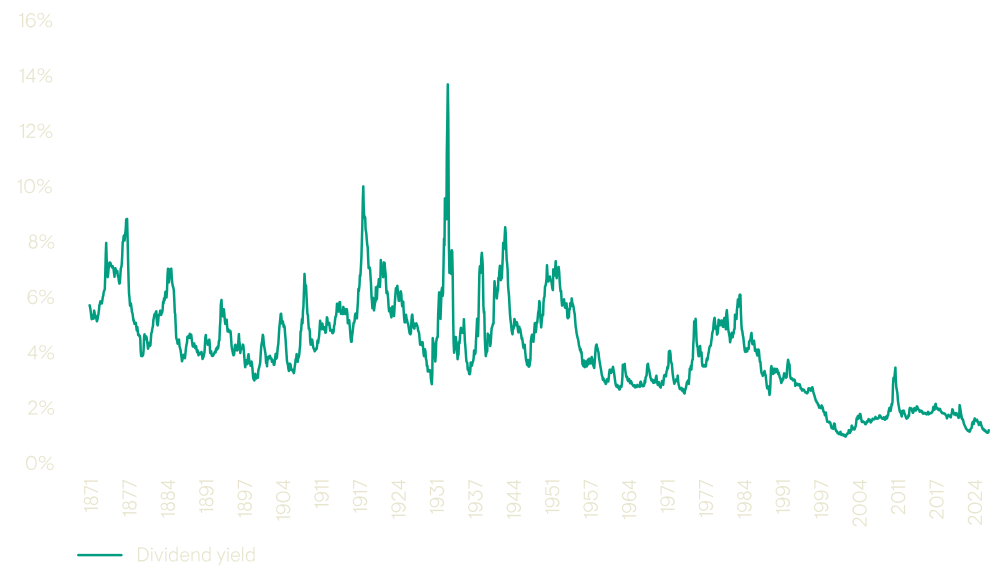
We proxy income with dividends. While many equity investors prefer to focus on earnings, we regard dividends as being less subject to manipulation – these distributions are a tangible payment, and the information is publicly disclosed – and therefore more reflective of the long-term fundamental cash-generating properties of the broad market. While other metrics (e.g. free cash flow) have evolved, they do not yet have similarly long history.
Figure 17: The history of US dividends stretches back over a century
Source: Shiller, U.S. Stock Markets 1871-Present and CAPE Ratio.
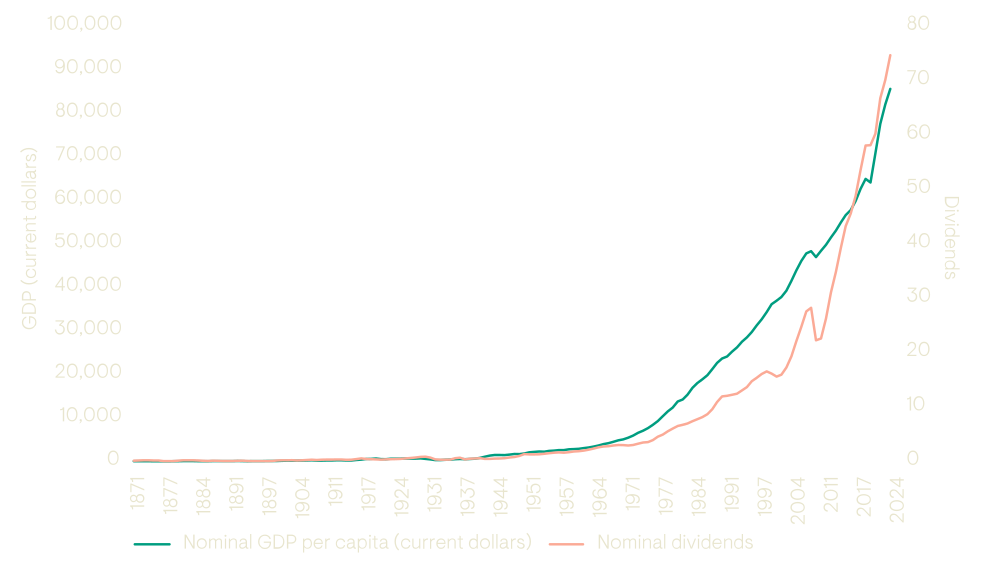
In this context, growth primarily relates to an equity market’s ability to increase dividends over time. GDP per capita has historically proven to be a reasonable proxy for dividend growth – and a closer match than GDP itself, as illustrated in the next chart. We simply allow for the global effects of growth based on the extent of non-domestic revenue exposure, assuming developed market growth is an average of local and global growth, while emerging market growth is wholly determined locally9. Growth is proxied based on trailing 15-year trend growth, a period that captures the secular effects of a couple of cycles. We apply a market adjustment factor – which includes changes in market composition relating to primary and secondary issuance, M&A activity, buybacks, new index inclusions etc. In each case, an owner of the market would have to either inject or remove capital to remain fully invested.
Figure 18: Nominal GDP per capita has proved a useful proxy for dividend growth
Source: Shiller, U.S. Stock Markets 1871-Present and CAPE Ratio; Louis Johnston and Samuel H. Williamson, “What Was the U.S. GDP Then?” MeasuringWorth, 2025.
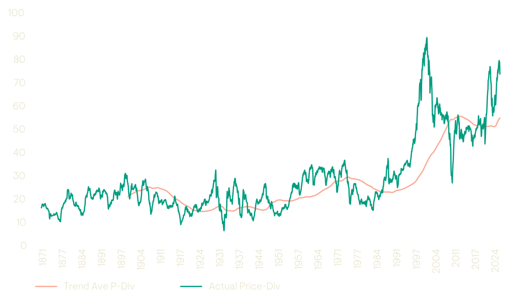
Lastly, we factor in an adjustment for revaluation. We believe that valuation acts as a gravitational pull over long periods; however, changes in market composition and dynamic means that this is not a static metric. We use the price-dividend ratio and trend dividend yield as our valuation metric, assuming this reverts to a long-term (15-year) average. This allows us to both maintain consistency with our income-focused framework, and smooth out the cyclical nature of dividends. While we acknowledge full reversion is unlikely – prices tend to overshoot both on the upside and the downside – this simplification remains conceptually sound on average, as can be seen in Figure 19.
Figure 19: The actual price-dividend reverts reasonably neatly to the trend average over time
Source: Shiller, U.S. Stock Markets 1871-Present and CAPE Ratio, internal calculations.
Fixed Income
Our portfolios target specific duration contributions when allocating to bonds; therefore, we feel it appropriate to use constant maturity bonds as the basic building block. We further deconstruct bonds into risk- free and spread components, enabling us to cover both sovereign and corporate debt.
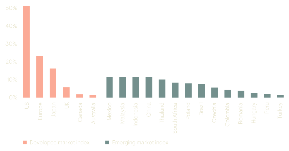
Income assumes the par yield of the bonds, typically for a notional 10-year bond. Regional indices are then generated by using the weighted average of the relevant market inclusions, as illustrated below.
Figure 20: Regional indices are generated using a weighted average of the relevant countries
Source: Ninety One calculations. Weights based on JP Morgan indices.
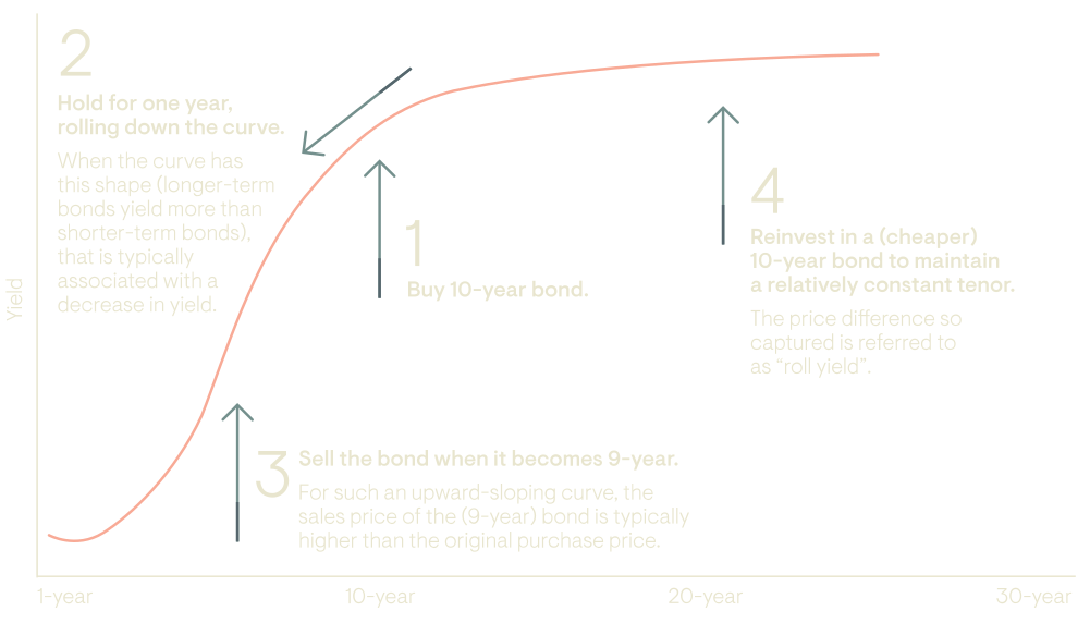
We define growth as being the roll yield obtained from consistently rebalancing the portfolio to maintain a constant maturity. So, for example, with a typical contango yield curve where the longer-term price is higher than the short-term, after one year the bond holder would sell the lower yielding, higher priced nine-year bond to buy a higher yielding, lower priced 10-year bond. Implicit in this view is a belief that the shape of the yield curve remains relatively consistent (including a constant spread component for credits).
Figure 21: Growth is the roll yield from consistently rebalancing the portfolio to maintain a constant maturity
Source: Ninety One. This graphic is for illustrative purposes only.
Revaluation is easier for government bonds than corporates; the former typically have liquid, traded markets enabling us to infer the forward market expectation of pricing. The implicit belief that markets converge to these expectations seems reasonable as a baseline for active management decisions.
Currency
We calculate currency returns in local currency. As explained in the currency section, we then adjust on two bases:
Hedging
Since it is common practice to hedge currency risk, and these costs are largely known at the date of investment, we use this as our base case. We assume that the position is hedged at inception for the 10-year horizon (essentially ignoring the small cash-flow differences that might occur), using covered interest rate parity. We derive the relative hedging cost from the zero coupon bond yields corresponding to the investment horizon.
Conversion
Many investors are willing to bear the currency risks, and therefore hold their assets unhedged. To proxy this, we use real effective exchange rates – i.e. adjusting the currency cross rates for relative inflation movements. We assume these exchange rates revert to their 15-year averages with an allowance for the difference in inflation targets, thereby allowing some currency mean reversion.
9 Based on the Morgan Stanley Global Exposure Guide 2022, Developed Markets tend to average c. 40% foreign exposure, while Emerging Markets are roughly 25%.
Frequently asked questions
To foster a sense of dialogue, we include a curated list of questions we have received from various stakeholders and our responses. We will continue adding to this section over time.
Q In equities, why have you used GDP per capita and not GDP itself?
GDP per capita has historically proven to be a reasonable proxy for dividend growth.
This is even though the relationship between fundamental company growth, in aggregate, and country-level economic growth is weaker than might otherwise be expected due to compositional mismatches. For example, GDP includes both private and public sector outputs; however, only the former are captured in aggregate via listed equities. Similarly, economic growth tends to be locally focused whereas listed companies often have substantial global operations.
Q What assumptions do you make for credit defaults?
We make allowances for credit defaults with the bond growth rate, using Moody’s long-term default histories. We use the Moody’s country rating for specific country sovereign debt, and the ratings banding for credit indices. By assuming that a AAA rating has similar meaning in both sovereign and corporate contexts, we can reasonably proxy a wide array of indices. (Based on history, we have applied an additional default factor for sub investment grade sovereign debt).
Q Why nominal (and not real) returns?
Inflation is notoriously difficult to predict; so much so, that our work suggested that nominal forecasts were often more reliable than real forecasts.
Q Why two currency bases – hedged and converted?
Both are common approaches to international exposure – some prefer hedging, whereas others are prepared to bear the resultant currency risk. We therefore thought it appropriate to include both so, irrespective of preference, the assumptions would be useful.
Q How are Capital Market Assumptions used within the Multi-Asset process?
Capital Market Assumptions are a framework for thinking about reasonable client outcomes and providing broad market context. These figures do not directly result in individual investment decisions.
Importantly, the Capital Market Assumptions represent the view of the Multi-Asset Capability within Ninety One; other investment teams are free to disagree.
Q Are the assumptions purely systematic?
We wish the framework to be consistent over time to help sharpen thinking on asset-level drivers; therefore, where possible, we prefer to use set assumptions.
We do, however, reserve the right to override specific assumptions where there is a strong market-specific reason to do so.
Q Why do you not predict macro-economic variables within the Capital Market Assumptions?
We wish to understand potential client outcomes over the long-term; therefore, our focus is on identifying those drivers which best explain and predict such outcomes. As can be seen in our framework, that can be done without specific macro-economic views.
Q Why do your growth assumptions look so much more pessimistic than the last twenty years of equity and/or dividend growth?
For corporate cashflows to continue growing at a significantly faster rate than the broad economy, one of three things needs to occur:
- Revenue grows faster than the broad economy – e.g. via the launch of new products which are far superior to competitors, or through the capture of new market segments. The former should not make a difference at the aggregate market level (one competitors revenue growth comes at the expense of another) but the latter may occur through, for example, internationalisation. That is why we link growth to a mixture of local plus global GDP.
- Costs fall (or, equivalently, margins increase) – e.g. via lower tax rates, more efficient use of resources, economies of scale, or regulatory capture. We think further margin expansion is challenging as tax decreases have likely reached their nadir, while regulatory capture cannot happen indefinitely. Since we have not yet found a reasonable long-term (10-year) predictive proxy, we prefer not to forecast this element, i.e. assuming that margins remain roughly constant.
- Business reinvestment increases (when returns are higher than the cost of capital) – If businesses are prioritising their investment, marginal investments will offer a decreasing rate of return, such that ultimately returns converge to cost of capital. If not, we’d expect competitors to enter. Again, a natural limit exists. Again, in the absence of a reliable predictive proxy, we essentially assume that pay-out ratios remain constant.
In short – because we focus on variables that have both been historically predictive and have a sensible fundamental interpretation, we continue to favour GDP as a predictor (implicitly, of revenue). We continue to actively research appropriate variables for margins and pay-out ratios; however, in an environment where we think each faces headwinds, we are comfortable to continue with our simplifying assumption.
Q How often are your assumptions updated?
We intend to update the Capital Market Assumptions twice each year – after the March and September quarter-ends.
We may also provide intra-period updates if we believe a market event is significant enough to materially change the 10-year outlook. For example, we released an internal update in late March 2020 to highlight the potential upside from equities and credit after the initial COVID-induced market collapse.
Q What is an index divisor and what causes this value to change?
The index divisor is defined as:
Index divisor = Index market cap/Index price
The index divisor is central to the calculation of equity indices because there are corporate actions and compositional changes which affect the aggregate value or market capitalisation measured by the index, but which do not impact the performance of the index. When the market value of the index increases or decreases because of one of these events, the index divisor is adjusted to ensure that the price of the index remains unchanged.
The impact of specific corporate actions or compositional changes can be either positive or negative for future returns, but they are aggregated into a single overall value.
A non-exhaustive list of some of the corporate actions which impact the index divisor is given in the table below.
| Corporate action | Impact on index divisor | Impact on index returns |
|---|---|---|
| Share repurchase (buyback) | Negative | Positive |
| Rights issue | Positive | Negative |
| Stock-based compensation | Positive | Negative |
| IPO | Positive | Negative |
| Cash acquisition (of index constituent) | Negative | Positive |
| Spin-off (where spin co is not an index constituent) | Negative | Positive |
In addition, the composition of the index can change as a result of index rebalancing events where index rules determine that existing companies be added to or removed from an index or that the proportion of a company’s shares which are included in the index changes. For regional indices, whole countries may also be added or removed from the index.
Items such as buybacks tend to be stable – their attractiveness is based on the regulatory and taxation basis applicable at a point in time, which tend to change infrequently. Other sources may be more volatile – for example, market changes due to M&A activity, views on the appropriateness of stock-based compensation, or even secondary issuance due to market stress. We infer the market adjustment impact from the change in MSCI Index Divisor over time.
Q Have you considered the impact of issuance or other corporate activity on the growth of income within equities?
Broad economic growth drives the growth generated by the listed corporate sector over the long run. However, it is accepted that corporate action, including mergers, acquisitions, research, and innovation ensure that the corporate sector is dynamic, undergoing compositional changes over time.
Our process starts with an assessment of the aggregate growth of the dividends paid by this dynamic mix of businesses. The next step is to make a market adjustment to capture all the corporate actions and index composition changes which directly increase or decrease the total value of equity measured by the market index.
As defined, the market adjustment factor is important as it changes the participation in the aggregate dividend growth of the entire market for an ongoing investor in the index. Market adjustments at the index level are analogous to but not identical to the way that equity issuance and repurchases affect returns for a single stock. To understand this, we must first recognise that to receive the index return, an investor must build a portfolio which holds every stock in the index in their index weights and which adjusts these holdings over time as index composition and weights change.
Any corporate action or index composition change which adds new equity capital into the index therefore dilutes future index returns in the same way that a company making a rights issue dilutes returns for holders of that stock. In both cases, if an investor does nothing, their ownership of the index or of the stock declines and the proportion of future value creation which flows to their shares falls. On the flipside, any corporate action or index composition change which removes equity capital from the index is accretive to future returns in the same way that a company repurchasing and retiring existing shares is accretive.
Importantly, these effects only directly impact an investor who seeks to own the entire market as defined by the index provider. For an active investor who does not hold the companies which launch these corporate actions there is no direct impact on their returns although there may be indirect impacts because of related capital flows or changes in the competitive environment.
Q How effective have your Capital Market Assumptions been?
As can be seen in this analysis, the Capital Market Assumptions have shown clear differences between market troughs and market peaks.
Q Given that Capital Markets Assumptions have so much associated uncertainty, what is the benefit of even attempting?
We see two key benefits:
- A clear understanding of return drivers enables sharper thinking about potential asset class outcomes, including under various scenarios.
- Insight into the likely direction and possible magnitude of returns helps our clients understand what outcomes may be reasonable.
Q Why use dividends/price-dividend rather than earnings and the more conventional price/earnings?
Dividends, being physical payments to shareholders, are less subject to manipulation than earnings (which are only book profits). We believe that results in stronger conclusions.
In addition, data sets tend to have a longer history of dividend payments, enabling us to consider the approach in a broader variety of historic contexts.
Q What key factors are not considered in your approach?
Our Capital Market Assumptions assume that the fundamental market drivers remain unchanged. They therefore ignore exogenous shocks – e.g. climate risks and geopolitical events (although we may update our assumptions in the event of a material shock).
We currently focus on single-asset return outcomes; therefore, we make no comment about potential changes in cross-asset correlations or asset-specific volatilities.We do not adjust for individual client circumstances either: client tax status may impact the relative attractiveness of asset classes.
Q Why a 10-year horizon?
As long-term custodians of our client’s capital, our focus is on helping our clients achieve suitable outcomes.
In addition, we require a timeframe long enough for fundamental drivers to be expressed, despite cyclical noise.
Ask a question
If you have any questions about our framework that you'd like to discuss further, please complete this form and we will respond to you directly
General risks. Forecasts are inherently limited and modelling involves risks, assumptions and uncertainties, they are forward looking and are not guarantees nor a reliable indicator of future results. Actual returns could be materially higher or lower than projected. This information is not intended as a recommendation to invest in any particular asset class or strategy or as a promise of future performance. The value of investments, and any income generated from them, can fall as well as rise. Costs and charges will reduce the current and future value of investments. Where charges are taken from capital, this may constrain future growth. Past performance is not a reliable indicator of future results. If any currency differs from the investor's home currency, returns may increase or decrease as a result of currency fluctuations. Investment objectives and performance targets are subject to change and may not necessarily be achieved, losses may be made. Environmental, social or governance related risk events or factors, if they occur, could cause a negative impact on the value of investments.
Explore more insights

Insights
Market and portfolio insights, webinars & events curated from across our investment teams to help you steer through changing investment landscapes.
Important information
Source: Ninety One proprietary capital market assumptions as at 31 March 2025.
These estimates are gross of fees (returns can be reduced by management fees and other expenses incurred) and reflect the view of Ninety One’s multi-asset team, whilst the views of other teams across Ninety One may differ. Details on our Capital Market Assumptions methodology available upon request.
Our expected returns estimates are for illustrative purposes only, are not a guarantee of performance and are subject to change. They are provided merely as a framework to assist in the implementation of an investor’s own analysis and an investor’s own view on the topic discussed herein. They should not be relied upon as recommendations to buy or sell securities. Forecasts of financial market trends that are based on current market conditions constitute our judgment and are subject to change without notice. We believe the information provided here is reliable, but do not warrant its accuracy or completeness. The outputs of the assumptions are provided for illustration/discussion purposes only and are subject to significant limitations. Expected return estimates are subject to uncertainty and error. Expected returns for each asset class are conditional on an economic scenario; actual returns in the event the scenario comes to pass could be higher or lower, as they have been in the past, so an investor should not expect to achieve returns similar to the outputs shown herein. Because of the inherent limitations of all models, potential investors should not rely exclusively on the model when making a decision. Unlike actual portfolio outcomes, the model outcomes do not reflect actual trading, liquidity constraints, fees, expenses, taxes and other factors that could impact the future returns. Note that these asset class assumptions are passive, and do not consider the impact of active management. All estimates in this document are in US dollar terms unless noted otherwise. The final total returns are converted from logarithmic to geometric estimates. This means that the components of the return breakdown may not sum to the total return. While useful for modelling and calculation purposes, the logarithmic return is theoretical (assumes continuously compounding returns) whereas the geometric estimate reflects practical experience (reflects discrete periods of compounded returns).
Indices
Indices are shown for illustrative purposes only, are unmanaged and do not take into account market conditions or the costs associated with investing. Further, the manager’s strategy may deploy investment techniques and instruments not used to generate Index performance. For this reason, the performance of the manager and the Indices are not directly comparable.
If applicable MSCI data is sourced from MSCI Inc. MSCI makes no express or implied warranties or representations and shall have no liability whatsoever with respect to any MSCI data contained herein. The MSCI data may not be further redistributed or used as a basis for other indices or any securities or financial products. This report is not approved, endorsed, reviewed or produced by MSCI. None of the MSCI data is intended to constitute investment advice or a recommendation to make (or refrain from making) any kind of investment decision and may not be relied on as such.
If applicable FTSE data is sourced from FTSE International Limited (‘FTSE’) © FTSE 2023. Please note a disclaimer applies to FTSE data and can be found here.
Global equities = MSCI All Countries World; Developed equities = MSCI World; US equities = MSCI USA; Continental Europe equities = MSCI Europe ex UK; Japan equities = MSCI Japan; UK equities = MSCI UK; Emerging equities = MSCI EM; China equities = MSCI China; Global sovereign bonds = Country-weighted composites, based on the JP Morgan Global Bond Index, of our regional estimates*; US, Europe, Japan, UK, China sovereign bonds = Notional 10-year bond; Emerging (Local Currency) bonds = Country-weighted composites, based on the JP Morgan GBI-EM Global Diversified, of our regional estimates*; US Investment Grade = Notional 10-year bond, using Bloomberg US IG Yield Curve; US High Yield = Notional 5-year bond, using ICE BAML US High Yield index for OAS; Sovereign Emerging (Hard Currency) = Notional 10-year bond using JP Morgan EMBI Global Diversified Index spread; Emerging Investment Grade = Notional 5-year bond using JP Morgan CEMBI Global Diversified Index spread.
*Not all of which are shown here.